Solving Sudoku via SAT with Mathematica
Introduction
A popular problem to write a program for is a Sudoku puzzle solver. Sudoku puzzles are relatively simple timewasters that many of us have solved on airplanes on paper and pencil (or pen if one is brave). The basic concept of a Sudoku puzzle is that one has a 9×9 grid that is broken into nine 3×3 subgrids. The goal is to find a marking of the 9×9 grid such that the numbers 1 through 9 appear without repetition in each column, row, and 3×3 subgrid. One starts with an initial marking, and has to fill in the empty squares with valid numbers until the puzzle is filled up. For easy problems, the initial marking makes it pretty easy to fill out the puzzle, but for harder ones with a relatively sparse initial marking, the process of filling out the puzzle can be challenging to do by hand.
A number of solver techniques can be used to attack the problem, such as classical tree search methods that explore the solution space and rule out markings that violate the problem constraints. In this example, we take a different approach and don’t actually write a solver. Instead, we take advantage of a very general type of solver known as a SAT solver, and show that by encoding a Sudoku puzzle as a SAT problem, the SAT solver can very rapidly generate a solution for us.
SAT solvers are very generic tools that are designed to solve what are known as boolean satisfiability problems. A satisfiability problem is one in which we start with a single large boolean formula and seek an assignment of truth values (true or false) to the variables in the formula such that the overall formula is true. If such an assignment can be found, we say that the formula is satisfiable and the solver can emit a set of variable assignments that yield this satisfying state. If the formula is not satisfiable, the solver will tell us that it is unsatisfiable (UNSAT). SAT solvers operate on boolean formulas in what is known as conjunctive normal form (CNF), where a formula is built as a set of smaller formulae made up of variables (or their negation) connected by OR operators, and these smaller formulae are connected by conjunction (AND) operators. Any boolean expression can be converted into CNF by the application of basic propositional logical laws such as De Morgan’s laws and others. Conversion of arbitrary boolean formulas to CNF is outside the scope of this document.
For those who have Mathematica and would prefer to follow along in the notebook file from which this post was derived, it is available in my public github repo here.
Encoding Sudoku
In this post, we will use the SAT encoding for Sudoku as defined in this paper. To express Sudoku as a SAT problem we must encode the state of the grid, as well as the constraints that define a valid marking. In essence, we are going to encode something along the lines of “position I,J is marked 3, position M,N is marked 5, …” for the entire grid, as well as the constraints on the rows, columns, and 3×3 subgrids that determine whether or not a marking meets the rules of the game. Since a SAT problem requires us to encode everything in terms of booleans instead of integers, we can’t simply say that “I,J is 3”. The encoding we discuss here takes the approach of stating that for position I,J, there are 9 boolean values corresponding to which of the 9 potential values are actually in the grid cell. If I,J is marked 3, then we would say that the variable corresponding to that (call it I,J,3) is true, while all others (I,J,1 and I,J,2 and so on up to I,J,9) are false. So, the state of the grid is represented as a 9x9x9 set of boolean variables – every possible position, and every possible value.
In Mathematica, we can create such a set of boolean variables by creating a 9x9x9 table of uniquely named variables.
The table S contains 9x9x9 uniquely named symbols that we can work with as our boolean values. At this point, they don’t have any truth value associated with them – they just denote the labels for the variables and the truth assignment will come later.
Before we proceed, we will create a couple of helper functions. One idiom that we want to work with are conjunctions or disjunctions over a list of formulae. For example, if we want to say “s1 AND s2 AND s3 AND s4”, it would be convenient to say “AND [s1,s2,s3,s4]”. This can be achieved by folding the appropriate operator (AND or OR) over a table, with the appropriate initial value for the fold.
Once we have this, we can start to set up the constraints that define the puzzle rules. The simplest constraint states that each cell has at least one value associated with it. So, cell x,y is either 1 or 2 or 3 or … or 9. That corresponds to a disjunction of the variables x,y,1 and x,y,2, and so on. Since this then applies for all possible instances of x,y, each set of disjunctions is joined with a conjunction. This is easily implemented with our helpers.
f1 =
 AndList[Table[
   AndList[Table[
     OrList[Table[
       s[[x, y, i]],
     {i, 1, 9}]],
   {x, 1, 9}]],
 {y, 1, 9}]];
Now, the rules also state that each value occurs at most in each row and each column, which we capture in formula f2 and f3.
f2 =
 AndList[Table[
   AndList[Table[
     AndList[Table[
       AndList[Table[
         Not[s[[x, y, z]]] || Not[s[[i, y, z]]],
       {i, x + 1, 9}]],
     {x, 1, 8}]],
   {z, 1, 9}]],
 {y, 1, 9}]];
f3 =
 AndList[Table[
   AndList[Table[
     AndList[Table[
       AndList[Table[
         Not[s[[x, y, z]]] || Not[s[[x, i, z]]],
       {i, y + 1, 9}]],
     {y, 1, 8}]],
   {z, 1, 9}]],
 {x, 1, 9}]];
Formula f4 and f5 capture the final constraint that states that each number appears at most once in each 3×3 subgrid. These are more complex since we need to repeat the constraints for each subgrid. The inner portion of the constraint deals with a single 3×3 subgrid, and the conjunctions outside that iterate those inner constraints over the full set of 3×3 grids. While this looks potentially complex due to the deep nesting of constraints, writing the indices out by hand makes it pretty clear.
f4 =
 AndList[Table[
   AndList[Table[
     AndList[Table[
       AndList[Table[
         AndList[Table[
           AndList[Table[
             Not[s[[3 i + x, 3 j + y, z]]] ||
             Not[s[[3 i + x, 3 j + k, z]]],
           {k, y + 1, 3}]],
         {y, 1, 3}]],
       {x, 1, 3}]],
     {j, 0, 2}]],
   {i, 0, 2}]],
 {z, 1, 9}]];
 f5 =
 AndList[Table[
   AndList[Table[
     AndList[Table[
       AndList[Table[
         AndList[Table[
           AndList[Table[
             AndList[Table[
               Not[s[[3 i + x, 3 j + y, z]]] ||
               Not[s[[3 i + k, 3 j + l, z]]],
             {l, 1, 3}]],
           {k, x + 1, 3}]],
         {y, 1, 3}]],
       {x, 1, 3}]],
     {j, 0, 2}]],
   {i, 0, 2}]],
 {z, 1, 9}]];
Once we have done this, we can look at the size of the constraint set.
As we expect from the paper that describes this encoding, we should have a formula with 8829 clauses. At this point we can move on to encoding the initial marking of the puzzle as additional constraints. Once we do that, we can let the SAT solver loose to find an assignment of truth variables such that all constraints (rules and initial marking) hold, which means the puzzle is solved. I decided to encode the initial markings as an associative array that maps coordinates to markings. So, the association of {3,5} to 4 means that at position {3,5} in the grid a 4 has been written in the box. Here is the marking for a simple Sudoku puzzle.
initial = <|
 {1, 2} -> 6, {1, 3} -> 1, {1, 4} -> 8, {1, 9} -> 7,
 {2, 2} -> 8, {2, 3} -> 9, {2, 4} -> 2, {2, 6} -> 5, {2, 8} -> 4,
 {3, 5} -> 4, {3, 7} -> 9, {3, 9} -> 3,
 {4, 1} -> 2, {4, 4} -> 1, {4, 5} -> 6, {4, 7} -> 3,
 {5, 1} -> 6, {5, 2} -> 7, {5, 8} -> 5, {5, 9} -> 1,
 {6, 3} -> 4, {6, 5} -> 2, {6, 6} -> 3, {6, 9} -> 8,
 {7, 1} -> 7, {7, 3} -> 5, {7, 5} -> 9,
 {8, 2} -> 9, {8, 4} -> 4, {8, 6} -> 2, {8, 7} -> 7, {8, 8} -> 3,
 {9, 1} -> 1, {9, 6} -> 8, {9, 7} -> 4, {9, 8} -> 6|>;

ShowMarking[initial]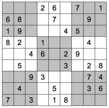
Once we have this, we can convert this to a boolean formula. This entails enumerating the symbols s[x,y,v] for all positions and values that are true as a list of variables connected by conjunctions.
At this point, we’re done! Solving the problem is a matter of asking whether or not a satisfying instance exists for the constraints AND the initial marking. So, we conjoin all of the constraints and the initial marking, as well as the full list of symbols that appear in the formula, and let the solver go.
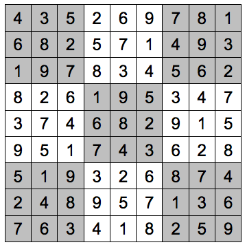
What returns is a list of boolean assignments for all of the symbols that were passed in, which in this case is the 9x9x9 array of symbols corresponding to all possible markings. We will need to reshape the flattened 999 long list into a 9x9x9 cube.
Once we have done this, we can then visualize the answer. The core of this is the Position function which is applied to the 9 element long list for each cell that corresponds to the marking of the cell. Specifically, the entry in that list that is true indicates which value to write in the cell of the puzzle. So, if XY4 is true, that says that the cell XY has a 4 in it.
    { {4, 6, 1, 8, 3, 9, 5, 2, 7},
      {3, 8, 9, 2, 7, 5, 1, 4, 6},
      {5, 2, 7, 6, 4, 1, 9, 8, 3},
      {2, 5, 8, 1, 6, 7, 3, 9, 4},
      {6, 7, 3, 9, 8, 4, 2, 5, 1},
      {9, 1, 4, 5, 2, 3, 6, 7, 8},
      {7, 4, 5, 3, 9, 6, 8, 1, 2},
      {8, 9, 6, 4, 1, 2, 7, 3, 5},
      {1, 3, 2, 7, 5, 8, 4, 6, 9} }
If we want to look at the puzzle in its usual grid form, this is pretty easy in Mathematica.
Once we have this methodology defined, it becomes easy to solve harder problems. Here is an assignment that is much harder to perform by hand since it is much sparser.
initialHard = <|
 {1, 6} -> 6, {1, 8} -> 5,
 {2, 1} -> 2, {2, 3} -> 7, {2, 5} -> 8,
 {3, 3} -> 4,
 {4, 2} -> 6, {4, 6} -> 5,
 {5, 3} -> 8, {5, 5} -> 4, {5, 7} -> 1,
 {6, 4} -> 3, {6, 8} -> 9,
 {7, 7} -> 7,
 {8, 5} -> 1, {8, 7} -> 8, {8, 9} -> 4,
 {9, 2} -> 3, {9, 4} -> 2|>;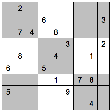
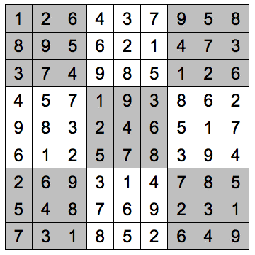
The SAT solver has no trouble with it, and yields the following solution.
Hopefully this shows some of the power of SAT solvers for solving general problems. Many problems can be written in terms of boolean satisfiability, and as soon as we do that we can take advantage of powerful SAT solvers. Beyond the one included in Mathematica, there are other popular SAT solvers such as MiniSAT and those embedded in more powerful tools known as SMT (Satisfiability Modulo Theories) solvers like Z3, Yices, and so on.
Helpers
For those who are curious, here are the helper functions used to show the solutions as well as the initial markings.
ShowSolution[soln_] :=
 Module[
   {rarray, r},
   r = ArrayReshape[soln, {9, 9, 9}];
   rarray = Table[Table[Flatten[Position[r[[i, j]], True]][[1]],
                  {j, 1, 9}], {i, 1, 9}];
   Graphics[
     Table[
      {EdgeForm[Thin],
       If[EvenQ[Floor[(j - 1)/3] + Floor[(i - 1)/3]*3],
         Lighter[Gray, 0.5],
         White],
       Rectangle[{i, j}, {i + 1, j + 1}],
       Black,
       Text[Style[rarray[[i, 10 - j]], Large], {i + 0.5, j + 0.5}]},
     {i, 1, 9}, {j, 1, 9}]
   ]
]ShowMarking[marking_] :=
Module[
{},
Graphics[
Table[
{EdgeForm[Thin],
If[EvenQ[Floor[(j - 1)/3] + Floor[(i - 1)/3]*3],
Lighter[Gray, 0.5],
White],
Rectangle[{i, j}, {i + 1, j + 1}],
Black,
If[KeyExistsQ[marking, {i, 10 - j}],
Text[Style[marking[{i, 10 - j}], Large], {i + 0.5, j + 0.5}]]},
{i, 1, 9}, {j, 1, 9}]
]
]