Comparing trees, functionally
In searching for ideas to write about for the F# advent calendar this year, it dawned on me that it was appropriate to write something about trees given the time of year.

One of the big attractions to functional programming for me is the clear conceptual mapping from abstract algorithm to code I personally find comes with the functional approach. So, today I’ll share one of my favorites that came from some work I did for a project in program analysis. For the curious, we applied this algorithm (albeit a Haskell version in a paper published at workshop a couple years ago for analyzing source control repositories. There is more to the code for that paper than summarized here, but the tree edit distance algorithm described below is at the core of it all.
One of the classical problems in computer science is the edit distance problem - given two strings, what is the minimal sequence of edits (insertions, deletions, or substitutions) that must be performed to one of them in order to yield the other? A common approach to solving this problem efficiently is to use an algorithm based on dynamic programming. For those who have forgotten that part of algorithms class, dynamic programming is often used in problems where greedy approaches fail to find the optimal answer. Basically, these are problems where a locally sub-optimal decision is necessary to find a globally optimal answer.
Not all structures of interest are equivalent to one-dimensional strings, so traditional string edit distance algorithms aren’t really useful when it comes to comparing them. An example of such a structure is a tree, either a plain old binary tree or a more general rose tree. Fortunately, the general algorithmic approach of dynamic programming can be used to compare trees too! One such algorithm was published in 1991 by Wuu Yang in an article entitled Identifying syntactic differences between two programs". In this post we’ll build out a function using this algorithm that takes two trees and a label comparison function that yields a pair of “edit trees” that correspond to the sequence of operations necessary to turn one of the inputs into the other (and vice versa).
Yang’s algorithm is essentially a recursive application of a traditional sequence edit distance algorithm applied at each level down the tree. The set of allowed edits is either keeping or deleting each subtree - unlike other edit distance algorithms, there is no substitution operation used. Edits are considered at each level of the tree, where the root is the first level, the children of the root are the second level, and so on. The algorithm seeks to find the best matching of the sequence of children directly below the subtree root, and recursively applies this to each of these subtrees. To illustrate a simple example of this, consider the trees below:
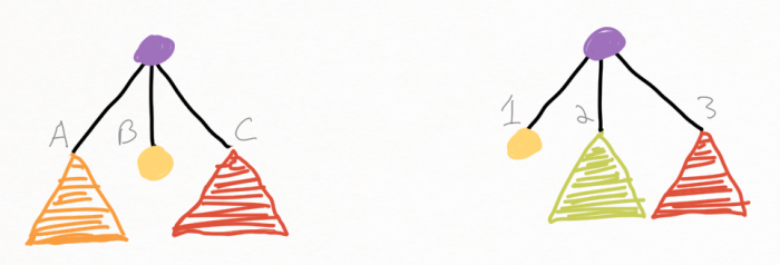
In this case, the color of the subtrees indicates equivalence - the red ones are the same, but the orange and green ones are unique to each tree. Similarly, the purple and yellow nodes appear in each tree. The edit sequence therefore corresponds to keeping the root level vertices (the purple one), and then at the second level, keeping the yellow vertex, discarding the orange subtree from the first tree and the green subtree from the second tree, and keeping the red subtree in both. The nodes at each level are considered to be ordered, so if we were to swap the orange node and red subtree in one of the trees and not the other, the result would be to discard everything below the purple vertex since no pairing in the order given exists. Whether or not this would matter to an application depends on the semantics of the tree structure. Here we are only concerned with trees where the order of children of each node in the tree matters.
Dynamic programming involves the construction of a table of intermediate costs associated with a sequence of actions (e.g., deletion, insertion, modification) applied to two input sequences. The step after constructing this table is to build a path through it starting at one corner to the other that maximizes (or minimizes) the cumulative cost. If we are comparing two rooted subtrees, then we can associate each row of the table with the children of the first subtree root, and the columns of the table with the children of the second subtree root.
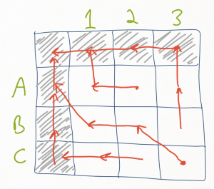
The path through the table starting from the lower right corner is composed of one of three actions: moving diagonally from the (x,y) coordinate to the (x-1,y-1) coordinate, moving left to (x-1,y), or moving up to (x,y-1). These moves correspond to maintaining both the xth child of the first tree root and the yth child of the second tree root, deleting the yth child of the second tree root (making no choice about the xth child of the first tree root yet), or deleting the xth child of the first tree root (and making no choice about the yth child of the second tree root yet).
So, how do we get started building this out in F#? For those who want to follow along with the full code available, it can be found on github. Our goal will be to build a function that implements Yang’s algorithm with the following type:
This function takes two trees, a function to compare the contents of the trees, and yields a pair - the quantitative edit distance score followed by a pair corresponding to the edit sequence to apply to the first tree and the edit sequence to apply to the second.
First, we can start encoding the decision making process for traversing the table that will eventually be built. I typically start by defining types of use in modeling the algorithm.
These can be related via a function that converts a direction to the corresponding actions to the first tree and the second tree. An option type is used to indicate whether we definitively do something (keep or delete) or make no choice yet.
let dirToOp = function
  | Up   -> (Some Delete, None)
  | Left -> (None,        Some Delete)
  | Diag -> (Some Keep,   Some Keep)
This corresponds pretty clearly to the text above - diagonal move, keep the element from both. A horizontal or vertical move corresponds to deleting from one tree, but deferring the decision about the element in the other tree until later along the path.
We need some trees to work with, so we can define a simple rose tree structure where each node of the tree is represented as a generic label type with a list of children. In F# speak, this type is an instance of a record.
Now, what do we need to encode in the table itself? At each cell, we need to know what the cost is so far, the direction to go from that cell, and something about the subtrees x and y under consideration at that point. As such, the table will be composed of cells containing a tuple of three elements - an integer, a direction, and a pair of indicators for how to interpret the xth and yth subtrees. In a common pattern in dynamic programming algorithms, we will have a special 0th row and 0th column of the table that acts as a sort of “gutter” that essentially encodes how to deal with the case where we’ve run out of contents for one of the sequences but not the other and want the algorithm to fall straight towards the (0,0) coordinate. These are indicated in the picture above as the cells with grey shading.
Let’s consider two cases: we are either dealing with a pair of subtrees to compare inside the table (x,y) where x>0 and y>0, or we are dealing with a location in one of the gutters (x,0) or (0,y). How do we interpret those? If we are inside the table, the subtree represented at that point has a root (of type ’a) and a list of children, each of which is a tree containing labels of type ’a. As we recurse down the tree, we determine whether or not these children would be deleted or kept. So, each cell of the table contains the root and a list of children where each child is a pair : an edit operation, and the corresponding tree. On the other hand, in the gutters we know that one of the sequences has been exhausted and the other isn’t going to be interpreted any further. The exhausted tree can be represented as a terminal element, and the tree that isn’t going to be interpreted any further can be treated as a leaf of the corresponding tree of edits where the entire subtree hangs off of the leaf.
This can all be encoded as the following type where an ENode corresponds to a rooted subtree with edits amongst its children, an ELeaf corresponds to a subtree below which no edits will take place, and ENil represents the terminal element for an exhausted tree:
To start off in creating the table we first want to map our inputs, which are two trees (ta and tb) each with a list of subtrees into an array of subtrees (call them ak and bk for “a kids” and “b kids”). This is because we want to have constant time lookup of any element, so an array is a natural way to do that. We’ll also create variables to hold their lengths to make the rest of the code a bit cleaner to read.
let ak = Array.ofList (ta.children)
let bk = Array.ofList (tb.children)

let lena = Array.length ak
let lenb = Array.length bk
Now, we want to initialize the array to some reasonable default value, so we will choose the tuple (0, Diag, (ENil, ENil)). All possible traces through this basically result in empty trees with a zero score.
As we work our way through the table, at any index ij, we are going to want to look at the table entry for (i-1)(j-1), i(j-1), (i-1)j. In addition, depending on what part of the algorithm we are at we may want to look at the score, the direction, or the pair of edit trees at that cell. Through the use of custom infix operators, we can avoid having our code peppered with a mixture of indexing logic and tuple unpacking by encapsulating it in functions.
Now, this is one of those parts of the code I thought hard about because custom infix operators are a mixed choice - on the one hand, they can make code very compact (which is my goal here), but on the other hand, they can be absolutely obtuse to read for someone who didn’t write the code in the first place. My rule of thumb is that I will use them in contexts within a function or module in a way where they cannot escape outside that context. In this case, when you look at the full function that we are defining, you’ll see that they are only visible within that single function. To me, that’s acceptable since a third party won’t have to look far for their definition.
In any case, let’s define three infix operators:
let (@!@) i j = let (a,_,_) = ytable.[i,j] in a
let (@+@) i j = let (_,b,_) = ytable.[i,j] in b
let (@%@) i j = let (_,_,c) = ytable.[i,j] in c
Each of these look up the i,j’th cell and return one element of the tuple. We’ll see why this is useful very soon. We can finally define the elements of the dynamic programming table:
for i = 0 to lena do
  for j = 0 to lenb do
    match (i,j) with
      | (0,0) -> ytable.[i,j] <- (0, Diag, (ENil, ENil))
      | (0,_) -> ytable.[i,j] <- (0, Left, (ENil, ELeaf (bk.[j-1])))
      | (_,0) -> ytable.[i,j] <- (0, Up,   (ELeaf (ak.[i-1]), ENil))
      | (_,_) -> let (ijscore, (ijl, ijr)) = yang (ak.[i-1]) (bk.[j-1]) lblcmp
                 let a = ( (i-1 @!@ j-1) + ijscore, Diag, (ijl, ijr) )
                 let b = ( (i-1 @!@ j  ),           Up,   (ijl, ijr) )
                 let c = ( (i   @!@ j-1),           Left, (ijl, ijr) )
                 ytable.[i,j] <- maxByFirst [a;b;c]
That’s it. The rest of the function is a bit simpler. Once we have the table defined, a dynamic programming algorithm will trace the optimal path through the table using the decisions that were made at each cell.
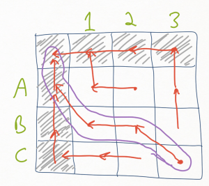
When processing cell (x,y), we want to interpret the move to make (up, down, diagonal), the edit trees that were stored in that cell for the xth and yth subtrees, and the coordinates of the cell along the trace path. We again make use of the inline functions to extract the second and third elements of the triplet at cell (x,y), and use pattern matching on the move direction to add an element to the traceback list and recurse. Due to the construction of the table (with the gutters), we set the base case to be (0,0) which corresponds to the empty list.
let rec traceback = function
  | (0,0) -> []
  | (x,y) -> let move = x @+@ y
             let (l,r) = x @%@ y
             match move with
             | Up    -> ((x,y), Up  , (l,r)) :: (traceback ((x-1), y    ))
             | Left  -> ((x,y), Left, (l,r)) :: (traceback (x,     (y-1)))
             | Diag  -> ((x,y), Diag, (l,r)) :: (traceback ((x-1), (y-1)))
The final step requires us to think about what we want this function to return. Given two trees, we want to return the score at that point as well as the list of edit trees corresponding to the children of the root of each tree. If we look at the list that is returned on the traceback, there are a few important properties to note:
- It’s backwards, since the list is built from the lower right corner to the upper left.
- The list of operations along the traceback is defined in terms of what we do to both sets of subtrees.
- When we map a direction to a pair of edit operations, the option type returned by dirToOp implies that some of points along the trace path we don’t have any information about what to do to one of the trees, so we would want to skip it.
- We want to pair up the edit operations with the corresponding edit subtree.
So, we want code that performs the traceback from the lower right corner, reverses the sequence, maps the direction at each step of the trace to a pair of edit operations that are associated with the pair of edit trees at that point in the tree, and then peels this list of pairs apart into a pair of lists.
let (tba, tbb) =
    traceback (lena, lenb)
    |> List.rev
    |> List.map (fun (_,d,(l,r)) -> let ops = dirToOp d
                                    ((fst ops,l),(snd ops,r)))
    |> List.unzip
This particular step may seem simple, but it represents a major advantage of languages like F# that provide an option type. In C# or other languages, we may simulate the option type with NULL values or something similar. Unfortunately, in those languages there is no way to distinguish the list that contains the NULLs and the list that does not. In F# on the other hand, the presence or absence of these is explicit via the option type. By having a mapping from the list with the optional values to a list without, we can guarantee that the list without them has no values of the None type. In languages in which we are dealing only with object references, the type system can’t help us separate code where we tolerate NULL values from code that does not. This is a very compelling feature of languages with Option types in my opinion (or, for the Haskellers out there, the Maybe type).
Looking at the function above, we can see one of my favorite parts of F# and related languages - the code is not hugely different than the description of what it is supposed to do.
Finally, we can spin through each of these lists to purge all of the steps in which the direction yielded a None operation, and at the same time unpack the Some instances to get rid of the option type.
let removeNones = List.choose (fun (x,y) -> match x with
                                            | Some s -> Some (s,y)
                                            | None   -> None)

let aekids = tba |> removeNones
let bekids = tbb |> removeNones
Now, finally we can define the score, and bundle the two lists of edit trees with the root of each tree to return the score and pair of edit trees. The score is either 0 if the roots don’t match, otherwise it is one plus the score at the lower right corner of the dynamic programming table. Given that the tree type is polymorphic in terms of the contents of the tree, we will use a comparison function that is passed in. This could also be accomplished by making the type parameter of the tree have a constraint that it be comparable - I chose not to do that, and don’t remember why (I wrote this code a few years ago).
The final bundling of return trees therefore is:
let (reta, retb) = if (score = 0) then (ELeaf ta, ELeaf tb)
                                  else (ENode (ta.label,aekids),
                                        ENode (tb.label,bekids))

(score, (reta, retb))
To see the code in action, one can play with the script in the repository that illustrates the sequence of edit actions described for the purple-rooted tree above. We start off with two trees, purp1 and purp2. [Edit 1/3/16: As a commenter somewhere pointed out, the subtrees for orange and green here have empty lists of children yet are illustrated as subtrees in the picture above. This makes no difference - because the root of each of these subtrees is where the mismatch occurs, what lies beneath them doesn’t change the result of applying the algorithm. I made a conscious choice to make them empty subtrees to avoid bloating up the code below. If one needs convincing, go ahead and check the code out and give it a try with non-empty subtrees for orange and green!]
val purp1 : Tree<string> =
  {label = "purple";
   children =
    [{label = "orange";
      children = [];};
     {label = "yellow";
      children = [];};
     {label = "red";
      children = [{label = "rchild";
                   children = [];}];}];}

val purp2 : Tree<string> =
  {label = "purple";
   children =
    [{label = "yellow";
      children = [];};
     {label = "green";
      children = [];};
     {label = "red";
      children = [{label = "rchild";
                   children = [];}];}];}
When we invoke the tree differencing code as:
The result is the edit trees for each side. The first one looks like this:
val p1 : EditTree<string> =
  ENode
    ("purple",
     [(Delete, ELeaf {label = "orange";
                      children = [];}); (Keep, ENode ("yellow",[]));
      (Keep, ENode ("red",[(Keep, ENode ("rchild",[]))]))])
How do we read this? Given that the roots match, we are handed back an edit tree that is rooted with a purple node that has three child edit trees: a child that states that the orange subtree is to be deleted, the yellow subtree is to be kept, and the red subtree is to be kept. Similarly, the other edit tree looks like:
val p2 : EditTree<string> =
  ENode
    ("purple",
     [(Keep, ENode ("yellow",[])); (Delete, ELeaf {label = "green";
                                                   children = [];});
      (Keep, ENode ("red",[(Keep, ENode ("rchild",[]))]))])
In both cases, the result of applying the edits to the corresponding input tree would be a purple rooted tree with two children: a yellow node followed by a red subtree.
The code associated with this post can be found on github. The code that is related to the paper I mention at the beginning can also be found on github and sourceforge (yes, I know - sourceforge. Don’t ask why…), which includes the edit distance code as well as algorithms that consume the result of the edit distance algorithm to identify specific changes made in trees. Eventually I would like to port those algorithms over to F# since they are pretty useful.