Harmonic Motion Simulation

2011-08-27

The model described in this post is pretty simple. Recently I found a pointer to this page that demonstrated harmonic motion with a collection of pendulums of different lengths. The apparatus shown here is based on a system described by Richard Berg in the article “Pendulum waves: A demonstration of wave motion using pendula” from the American Journal of Physics, Volume 59, Issue 2, 1991. Here is the video from the Harvard page showing the apparatus at work.

It seemed like an interesting and simple physical system, so I decided to see if I could replicate it computationally. This is fairly basic physics - this system is probably early undergrad level physics and math, right around the time when you first encounter non-linear partial differential equations.

To start, let’s remember what the equation of motion is for a damped pendulum (using Newton’s notation for derivatives):

\[ \ddot{\theta} + \gamma \dot{\theta} + \frac{g}{l} sin(\theta) = 0 \]

In this equation, \(\gamma\) is the damping coefficient, g is gravitational acceleration, and l is the length of the pendulum. In the video shown at the end, we assume that the damping coefficient is zero, so our little computational pendulum exists in a vacuum. If you download the code and set it to a non-zero value, you will see a nice damping out of the motion over time as one would expect in reality due to air resistance.

In the simulation, the variable we are concerned with is \(\theta\):

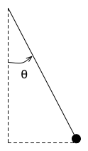
The second order partial differential equation that describes this system isn’t one that is easily solvable directly, so we resort to methods from numerical analysis to attack it. In this case, it is common to employ a fourth order Runge-Kutta scheme (see this document for a derivation of the Runge-Kutta scheme from the second order PDE). To start, we rewrite the equation in two parts:

\[ \omega = \dot{\theta} \]

\[ \dot{\omega} = -\gamma \omega - \frac{g}{l}sin(\theta) \]

Now that we have the system in terms of simultaneous first order equations, we can use the Runge-Kutta scheme to define a sequence of \(\theta\) and \(\omega\) values that are easily computable as:

\[ \theta_{n+1} = \theta_n + \frac{1}{6}(k_{1a} + 2k_{2a} + 2k_{3a} + k_{4a}) \]

\[ \omega_{n+1} = \omega_n + \frac{1}{6}(k_{1b} + 2k_{2b} + 2k_{3b} + k_{4b}) \]

Where we have the four coefficients for each defined for a time step \(\Delta t\) as:

\[ k_{1a} = \omega_n \Delta t \]

\[ k_{2a} = (\omega_n + \frac{k_{1b}}{2}) \Delta t \]

\[ k_{3a} = (\omega_n + \frac{k_{2b}}{2}) \Delta t \]

\[ k_{4a} = (\omega_n + k_{3b}) \Delta t \]

And

\[ k_{1b} = f(\theta_n, \omega_n, t) \Delta t \]

\[ k_{2b} = f(\theta_n + \frac{k_{1a}}{2}, \omega_n + \frac{k_{1b}}{2}, t + \frac{\Delta t}{2}) \Delta t \]

\[ k_{3b} = f(\theta_n + \frac{k_{2a}}{2}, \omega_n + \frac{k_{2b}}{2}, t + \frac{\Delta t}{2}) \Delta t \]

\[ k_{4b} = f(\theta_n + k_{3a}, \omega_n + k_{3b}, t + \Delta t) \Delta t \]

where

\[ f(\theta, \omega, t) = -\gamma \omega - \frac{g}{l}sin(\theta) \]

At this point, writing the code is really straightforward. First, define f. One change that we will make is that we will also specify the length of the pendulum, l, as a parameter. This won’t impact the derivations above though - it just makes it easier later on to compose together the set of individual pendulums of different lengths to mimic what we see in the video.

g :: Double
g = 9.80665 -- gravitational acceleration = 9.80665m/s^2

f :: Double -> Double -> Double -> Double -> Double
f theta omega t l = (-gamma)*omega - (g/l)*sin(theta)

Note that the t value isn’t used. We keep it for completeness, given that f as formulated formally is a function of \(\ddot{\theta}\), \(\dot{\theta}\), \(\theta\), and t. Once we have this, we can then define the code that implements one step of the Runge-Kutta solver for a given time step dt:

dt :: Double
dt = 0.01

solve :: (Double, Double, Double, Double) -> (Double, Double, Double, Double)
solve (theta, omega, t, l) =
  (theta + (1/6)*(k1a + 2*k2a + 2*k3a + k4a),
   omega + (1/6)*(k1b + 2*k2b + 2*k3b + k4b),
   t', l)
  where
    t' = t + dt
    k1a = omega * dt
    k1b = (f theta omega t' l) * dt
    k2a = (omega + k1b/2) * dt
    k2b = (f (theta + k1a/2) (omega + k1b/2) (t' + dt/2) l) * dt
    k3a = (omega + k2b/2) * dt
    k3b = (f (theta + k2a/2) (omega + k2b/2) (t' + dt/2) l) * dt
    k4a = (omega + k3b) * dt
    k4b = (f (theta + k3a) (omega + k3b) (t' + dt) l) * dt

Now, the original video that inspired me to spend my Friday evening playing with this model included a set of pendulums of different lengths. The Berg paper describes the lengths as follows: the longest pendulum is intended to achieve X oscillations over a time period of T seconds. Each shorter pendulum should achieve one additional oscillation over that same time period. Now, we know that the time for one oscillation of a pendulum of length l is given by:

\[ t = 2 \pi \sqrt{\frac{l}{g}} \]

From this, we can derive an equation for the length of pendulum n (where n runs from 1 to N, for N pendula with the Nth longest):

\[ l_n = g\left(\frac{T}{2 \pi (X+(N-n))}\right)^2\]

In the Berg paper, X is 60 and T is 54 seconds, which we can then implement:

lengths :: Int -> Double -> Double -> [Double]
lengths n t l =
  let thelen curn = (t/((l+((fromIntegral n)-curn)) * 2.0 * pi))**2 * g
  in
      [thelen (fromIntegral i) | i <- [1..n]]

theta0 = pi / 8
omega0 = 0
npendu = 24
starts = map (\i -> (theta0, omega0, t, i)) (lengths npendu 54.0 60.0)

So, every pendulum starts at \(\theta = \frac{\pi}{8}\), and we have 24 pendulums that take on lengths corresponding to those in the paper.

In order to watch the code run and replicate (as best as possible with this simple simulation) the video, I wrapped this code with Gloss to add simple visualization capabilities. The code is pretty simple: I set up some constants to define the window size, and then convert the angle into (x,y) coordinates via \((x,y) = (l sin(\theta), -l cos(\theta))\) where l is the length of the pendulum being rendered.

-- window parameters
winWidth :: Int
winWidth  = 600

winHeight :: Int
winHeight = 600

-- circle radius
cradius   = 5

-- colors for the pendulum and the string
clr = makeColor 1.0 1.0 0.0 1.0
lineclr = makeColor 0.3 0.3 0.3 0.5

-- render one pendulum
renderPendulum :: (Double, Double, Double, Double) -> Picture
renderPendulum (theta, omega, t, l) =
  let x = double2Float $ l*sin theta
      y = double2Float $ -(l*cos theta)
      twidth = ((fromIntegral winWidth) / 2)-15
      theight = ((fromIntegral winHeight) / 2)-15
  in
    Pictures $ [
      Color lineclr $
        Line [(0,0), (x*twidth,y*theight)],
      Color clr $
        Translate (x*twidth) (y*theight) $
        Circle cradius ]

-- render the list of pendulums
renderPendulums ps = Pictures $ map renderPendulum ps

This is then called from the main function that sets up the initial conditions for each, and then uses the Gloss simulateInWindow function to do the animation. Note that we don’t use the time parameter of the simulateInWindow function, and control the time stepping using the dt value defined before.

main :: IO ()
main = do
  let niter = 1000
      theta0 = pi / 8
      omega0 = 0
      t = 0
      npendu = 15
      starts = map (\i -> (theta0, omega0, t, i)) (lengths npendu 54.0 60.0)
  simulateInWindow
    "Pendulums"
    (winWidth, winHeight)
    (1, 1)
    (greyN 0.1)
    120
    starts
    renderPendulums
    (\vp f m -> map solve m)

The result of this is shown in the video here.

If you are interested in playing with this code, you can find it in my public github repository. Enjoy playing with the pendula!