Functional gene expression programming
A couple of posts ago, I talked about a simple monte carlo simulation for diffusion limited aggregation. In this post, I’m going to talk about another algorithm that, at its heart, is based on random numbers. Unlike DLA though, this algorithm isn’t about simulating a physical system. Instead, it is about a method for solving optimization problems that are generally poorly suited to traditional numerical optimization techniques. This post describes an application of a library implementing the GEP method posed by Cândida Ferreira nearly 10 years ago. I started messing with GEP shortly after the paper “Gene Expression Programming: A New Adaptive Algorithm for Solving Problems” was published in the journal Complex Systems. The paper sat in a pile for a while, and about two years ago I picked it up again and started to implement it as a Haskell library.
The library, HSGEP, has been available on github for a few months, and has been kicking around on my laptop at home for a couple of years. A few people have come across it and used it (and contributed some code back to make it better!). I figured if I posted about it here, a few more interested people may play with it and help me improve it.
Optimization is all about minimizing (or maximizing) some function. Given a function f(x), we want to find the value of x that yields the smallest value of f(x). If we cannot assume that we have an analytical formulation for f (i.e., we don’t know how to write it down as a polynomial) or the ability to compute derivatives for f, solving this problem becomes challenging. All of the techniques that we know and love from calculus cease to apply. Evolutionary algorithms are a nice family of methods that are inspired by biological processes in which a notion of fitness drives the refinement of candidate solutions. The fitness determines which candidate solutions continue to be refined, and operations on the solutions allow us to combine parts of them to form new solutions to try in hopes that two OK solutions will, when combined, yield a better one. No notion of derivatives or other information about the function being optimized or the candidate solutions is necessary - all we need is a set of tests to evaluate how fit a candidate is, and a set of operations for building new candidates from old ones.
A familiar example of this kind of optimization problem to most readers is the case where we have only a set of data points and want to find the function that best fits them. This is usually called regression. The input is the set of data points (x,y), and the output is some function f that minimizes the distance
\[|f(x)-y|\]
over the set of input data points. Statistics gives a number of methods that allow us to find these functions when they are of a certain class, like linear regression and nonlinear regression. Things get complicated when we don’t know in advance what the properties of the function that best fits our data are. What if we want to find a function that fits the data that may be quadratic, cubic, or possibly include a mixture of quadratics and logarithms or transcendentals? How do we search for a good fit? Even more interesting things occur when the optimization problem that we’re solving isn’t regression either. Regression is a nice, rather simple problem that can be used to introduce gene expression programming. For example, here is set of input points:
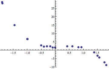
We would like to find a polynomial that is built up out of primitive operators like +, -, *, /, and the variable x. In the plot above, the data points are sampled from the following function with random noise added to each point.
\[ f(x) = 2+\frac{x}{2} + 2x^2 - 3x^3 \]
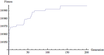
Our goal is to find this function given only the input data points. Using GEP we can evolve expressions until we find one that gets as close as it can to our data. Looking at the following plot of fitness values, we can see that after around 150 generations, we have reached a point near the maximum fitness (in this case, 19000). The individual isn’t perfect, primarily due to the fact that we added noise to the input data.
If we look at a few of the individuals that were produced, we can see that slowly but surely the individuals that improve in fitness get closer to the function that we are seeking. Three such examples are shown below. The yellow line is after 10 generations, green after 35, and purple after 200. The blue dots are the data points that we’re seeking a function that fits.
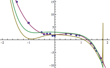
The functions corresponding to the yellow, green, and purple curves were:
\[ f_{10}(x) = 1+x-2x^2 +x^4 -x^5 +\frac{1}{1+x+x^2-x^3}\]
\[ f_{35}(x) = \frac{6-x+4x^2+2x^3-2x^4-2x^5+2x^6-2x^7}{2+2x^2}\]
\[ f_{200}(x) = 2+\frac{x}{2} + 2x^2 - 3x^3\]
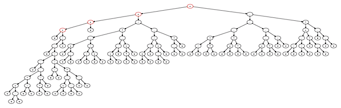
Of course, this was after simplification using a tool like Mathematica or Maxima. If you get a hold of the sources for hsgep, one of the bits of code I include is a small module to allow the code to call out to Maxima to simplify the final individual for pretty printing. Otherwise, you have to reason about expressions made out of the basic building blocks, like this (using ‘a’ as the variable, not x – the name doesn’t really matter):
((((a+((a-((a-(((a+(a-a))(a/a))-((aa)/a)))/((a/a)/(((a+a)-(a-a))(a-a)))))/a))+a)+((((a+(a-a))-((a/a)/(a+a)))(((a+a)-a)-((aa)+a)))/((((a+a)-a)/((a-a)+a))-((a-a)a))))+(((((a/a)(aa))-((a+a)(aa)))-(((a+a)-(aa))-(a/a)))-((((a/a)-(a/a))+(a(a-a)))*(a-(a-a)))))
This expands out to the expression tree here:
One of the appealing things about the library is that it isn’t very hard to add new functions to the set that can be used to build up the expressions. For example, if we add nonterminals for operations like square roots, logarithms, exponents, trig functions, etc., then we can explore a pretty rich space of complex functions. All this requires is adding them to the input parameter file that defines the genome, and then add them to the ArithmeticIndividual source file to make sure they are assigned the correct arity and interpreted properly during fitness evaluation. Included with the library are further examples of regression that use more than one variable as well.
If this looks interesting, I encourage you to go grab a copy of the code from either github or hackage. As time permits, I have a number of improvements to make to the library. Among them are:
- Moving the code to express a chromosome out of the example driver into the main library. The current location is an artifact of the early development of the code.
- Finishing the cellular automata density classification example. This is a second example from the original GEP papers, and I’d like to have a working version of it to accompany the library as an example.
- Parallelizing the code. Many opportunities for parallelization exist. For example, much of the time for the code is spent in the fitness evaluation stage. If the population is divided amongst the available cores, we should see a nice speedup due to the fitness evaluation problem being embarrassingly parallel.
- Tutorial for writing programs that use the library. Currently, one needs to infer how to do this by examining the regression or CAdensity examples. This really should be well documented.
- Adding plotting capabilities. The plots shown above for the fitness were performed using Mathematica. I’d like to use one of the plotting packages available on Hackage to accomplish this.
- Moving arity information out to the parameter file.
- Using a cleaner argument processing and parameter file reading capability.
Anyways, enjoy the library. Hopefully someone finds it useful or interesting. Keep an eye on the github page (or send me an e-mail) if you are interested in keeping up on the continuing development of the code.