Image Denoising by Regularization on Characteristic Graphs
Instead of a lengthy post like the last two, here’s a shorter one to give a pointer at a recently published paper.
T. Asaki, K. Vixie, M. Sottile, P. Cherepanov. “Image Denoising by Regularization on Characteristic Graphs” Applied Mathematical Sciences, Vol. 4, no. 52, 2010.
Download the PDF here.
This post has nothing to do with languages - just math and image processing. This paper was written with a few colleagues who were at Los Alamos with me when we did the work described in the paper. All of us have since moved on, Tom and Kevin to WSU, me to Galois, and Pavlo is still (to my knowledge) with UNM.
The abstract is:
This paper introduces improvements to a now classical family of image denoising methods through rather minimal changes to the way derivatives are computed. In particular, we ask, and answer, the question “How much can we improve the common denoising methods by local, completely non-parametric modifications to image graphs?” We present the concept of non-parametric characteristic graph representations of images and detail two such graph constructions. Their use in image denoising is demonstrated within a regularization framework. The results are compared with those of more traditional approaches of Tikhonov, total variation and L^1 TV regularization. We show that in some denoising scenarios our methods perform more favorably in preserving intensity levels and geometric details of object boundaries. They are particularly useful for denoising images with both smooth and discontinuous intensity variations, preserving detail to the pixel level.
The germ for this work came from some computational experiments that Tom and I were doing to see how graph-representations of images could help in segmentation problems. It turned out that, while not so useful in segmentation, our ways of looking at the images as graphs were useful for denoising. A fortunate bug in a graph traversal algorithm led to the first characteristic graph that we discuss in the paper, which led to thinking about the second.
Here is an example of the graphs:
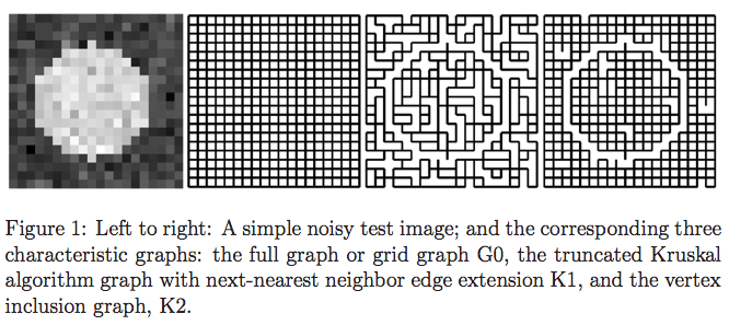
The far left image is the original image to be denoised. The next one is the full grid graph (G0) representing all of the connected pixels. The other two are the characteristic graphs that we introduce, K1 and K2. In this little illustration, I think K2 has some pretty obvious interesting properties just looking at it and the original image, don’t you think? K1 does as well, but given that K1 is sparser than K2, the “interestingness” isn’t as obvious to the naked eye.
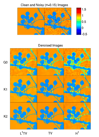
And here is a taste of the results. The bottom two rows are with the denoising method discussed in the paper. Instead of replicating the details here, I’d encourage people to take a look at the paper instead.