Finding dents in a blobby shape
Recently someone on a forum I read on researchgate.net posted a question: given some blobby shapes like:
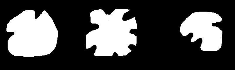
How do we find the number of indentations in each shape? A few years ago I was doing work with microscope slide images looking at cells in tissue, and similar shape analysis problems arose when trying to reason about the types of cells that appeared in the image.
Aside from any specific context (like biology), counting the dents in the black and white blobs shown above looked like an interesting little toy problem that wouldn’t be too hard to solve for simple shapes. The key tool we will use is the interpretation of the boundary of the shape as a parametric curve that we can then approximate the curvature along. When the sign of the curvature changes (i.e., when the normal to the curve switches from pointing into the shape to outside, or vice versa), we can infer that an inflection point has occurred corresponding to a dent beginning or ending.
The tools we need to solve this are:
- A way to find a sequence of points (x,y) that represent a walk around the boundary of the shape,
- A way to compute the derivative and second derivative of that boundary to compute an approximation of the curvature of the boundary at each point,
- A method for identifying dents as changes in the curvature value.
In Matlab, most of these tools are readily available for us. The bwboundaries function can take a binary image with the shape and produce the (x,y) sequence that forms the set of points around the boundary in order. The fast Fourier transform then can be used to turn this sequence into a trigonometric polynomial as well as computing derivatives necessary to approximate the curvature at the points along the boundary.
Working backwards, our goal is to be able to compute the curvature at any point along the boundary of the shape. We will be working with a parametric function defined as x=x(t) and y=y(t), which allows us to compute the curvature via:
\(\kappa = \frac{x'y''-y'x''}{\left( {x'}^2 + {y'}^2 \right)^\frac{3}{2}}\)
This means we need to have a way to compute the derivatives of the parametric function x’, x’‘, y’, and y’’. It turns out this is pretty straightforward if we employ the Fourier transform. A useful property of the Fourier transform is its relationship to derivatives of functions. Specifically, given a function x(t), the following property holds:
\(\mathcal{F} \left[ \frac{d^n}{dt^n} x(t) \right] = (i \omega)^n X(i \omega)\)
where:
\(X(i \omega) = \mathcal{F} [x(t)]\)
That relationship happens to be quite convenient, since it means that if we can take the Fourier transform of our parametric function, then the derivatives come with little effort. We can perform some multiplications in the frequency domain and then use the inverse Fourier transform to recover the derivative.
\(x^{(n)}(t) = \mathcal{F}^{-1}\left[ (i \omega)^n X(i \omega) \right]\)
Armed with this information, we must first obtain the sequence of points along the shape boundary that represent discrete samples of the parametric function that defines the boundary curve. Starting with a binary image with just a few dents in the shape, we can extract this with bwboundaries.
This function returns a cell array in the event that more than one boundary can be found (e.g., if the shape has holes). In the images considered here, there are no holes, so the first element of the cell array is used and the rest (if any are present) are ignored. The x coordinates are extracted from the second column of b, and the y coordinates from the first column. Now we want to head into the frequency domain.
As discussed above, differentiation via the FFT is just a matter of scaling the Fourier coefficients. More detail on how this works can be found in this document as well as this set of comments on Matlab central.
nx = length(xf);
hx = ceil(nx/2)-1;
ftdiff = (2i*pi/nx)*(0:hx);
ftdiff(nx:-1:nx-hx+1) = -ftdiff(2:hx+1);
ftddiff = (-(2i*pi/nx)^2)*(0:hx);
ftddiff(nx:-1:nx-hx+1) = ftddiff(2:hx+1);`
Before we continue, we have to take care of pixel effects that will show up as unwanted high frequency components in the FFT. If we look closely at the boundary that is traced by bwboundaries, we see that it is jagged due to the discrete pixels. To the FFT, this looks like a really high frequency component of the shape boundary. In practice though, we aren’t interested in pixel-level distortions of the shape - we care about much larger features, which lie in much lower frequencies than the pixel effects. If we don’t deal with these high frequency components, we will see oscillations all over the boundary, and a resulting huge number of places where the curvature approaches zero. In the figure below, the red curve is the discrete boundary defined by bwboundaries, and the green curve is the boundary after low pass filtering.
We can apply a crude low pass filter by simply zeroing out frequency components above some frequency that we chose arbitrarily. There are better ways to perform filtering, but they aren’t useful for this post. In this case, we will preserve only the 24 lowest frequency components. Note that we preserve both ends of the FFT since it is symmetric, and preserve one more value on the lower end of the sequence since the first element is the DC offset and not the lowest frequency component.
xf(25:end-24) = 0; yf(25:end-24) = 0;
The result looks reasonable.
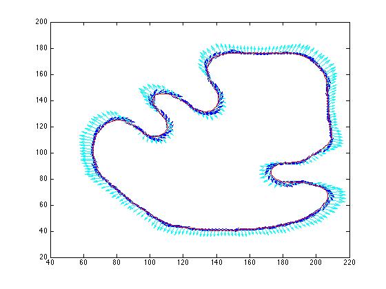
Finally, we can apply our multipliers to compute the derivative and second derivative of the parametric function describing the shape boundary. We only want the real components of the complex FFT.
dx = real(ifft(xf.*ftdiff'));
dy = real(ifft(yf.*ftdiff'));
ddx = real(ifft(xf.*ftddiff'));
ddy = real(ifft(yf.*ftddiff'));
Here we can see the derivatives plotted along the curve. The blue arrows are the first, and the cyan arrows are the second derivative.
Finally, we can compute our approximation for the curvature.
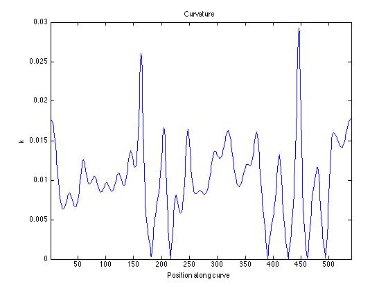
The last step is to identify places where the curvature approaches zero. Ideally, we’d be working with the signed curvature so that we can identify where inflection points are by observing the normal vector to the boundary surface switching from pointing outward to inward and vice versa. The approximation above is not signed, so we rely on another little hack where make the following assumption: the shape that we are dealing with never has flat edges where the curvature is zero. Obviously, this isn’t a good assumption in the general case, but sufficient to demonstrate the technique here. If this technique is applied in a situation where we want to do the right thing, the signed curvature is the thing we’d want to compute and we would look for sign changes.
Instead, we look for places where the curvature goes very close to zero, and assume those are our inflection points. Now, often more than one point near an inflection point exhibits near zero curvature, so we look for gaps of more than one point where the curvature is near zero. For each dent, we should see two inflection points - one where the boundary enters the dent, and one where it leaves it.
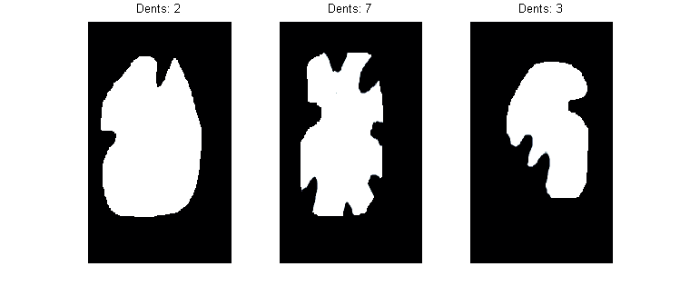
For the example images above, the code yields the correct number of dents (2, 7, and 3).
Before leaving, it’s worth noting some issues with this. First, the assumption that curvature diving towards zero implies that in the signed case it would have switched sign is definitely not valid in a general sense. Second, the filtering process is damaging to dents that are “sharp” - it has the effect of rounding them off, which could cause problems.
On the other hand, working with the boundary as a parametric curve and computing derivatives using the Fourier transform does buy us robustness since we stay relatively true to a well defined (in a mathematical sense) notion of what a dent in the shape is.