Playing with the Naming Game
Introduction
After reading a recent paper in Physical Review E, “Role of feedback and broadcasting in the naming game”, I decided to implement the model used in the paper just to play around with the algorithm and reproduce the results. Working through the rather simple algorithm, I realized that it would be an interesting little exercise to share.
The naming game is a simple model that was introduced a number of years in the article “A Self-Organizing Spatial Vocabulary” by L. Steels. It turns out that it captures features of distributed algorithms, such as distributed leader election, and allows analysis of properties of systems that implement these algorithms. People have looked at the model from the point of view of statistical physics in recent years – a number of articles on the topic are referenced by the recent Phys. Rev. E article for those curious about digging in deeper.
The model proceeds as follows. We start with a set of n entities, each of which know no words. Each time step, we pick two of these entities, and select one to be the speaker and the other to be the hearer. The speaker selects a word from the set of words that they know, and asks the hearer if they know the word as well. If the speaker knows no words, it invents a unique one and uses it. If the hearer doesn’t know the word, then it adds it to its dictionary. If it does know the word, then we have a few possible outcomes. In one outcome, both the speaker and hearer clear their dictionaries and only store the word that they have discovered someone else knows. In another outcome, the hearer clears their dictionary while the speaker keeps theirs full. Similarly, the third outcome is the one in which the speaker clears the dictionary, with the hearer keeping theirs intact.
It’s a simple model, and when we run it, we see interesting behavior like the following:
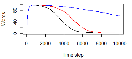
In this plot (made with GNU R), the x-axis represents time and the y-axis represents the number of unique words that exist in the population. The plots show the average number of words known within the population for 15 trials, each with 200 individuals over 10000 time steps. As we can see, there is a period of invention, in which a set of words are invented, followed by a long period over which time the population slowly converges on a single common word. In this case, we see all three update scenarios – the original rule in which both speaker and hearer clear dictionaries on agreement, red when the speaker is the one who clears, and blue when the hearer is the one who clears. These plots appear to agree with those in the paper, which means the little implementation I put together works.
Implementing this is pretty straightforward, but in doing so an interesting (albeit not very complicated) pattern emerges that can be elegantly dealt with in Haskell using the type system.
Consider the constraints of the model:
- Random number generation implies some changing state.
- Generation of unique new words efficiently also can be implemented via state.
- As the model runs, at each time step we care about logging the size of the world vocabulary.
- A set of parameters related to the model need to be accessed at various points in the code.
As usual, for those who wish to follow along and see all of the code (not all of it is posted here in the blog post), you can find it in the “ng” subdirectory of my public github repo.
Naive implementation
A first, quick and dirty implementation that I expected to run reasonably quickly was written by letting the C part of my brain drive, but using Haskell syntax. A simple data type was created in which IORefs are used to store mutable state:
One field of the record holds the state of the random number generator, and the other the counter used to generate new words. A set of simple functions is then responsible for manipulating values of this type.
newNGState :: IO NGState
newNGState = do
  r <- newIORef (mkStdGen 1)
  w <- newIORef 0
  return $ NGState { randState = r, wordState = w }

getInt :: NGState -> Int -> IO Int
getInt s n = do
  let randGen = randState s
  gen <- readIORef randGen
  let (val, gen') = randomR (0,(n-1)) gen
  writeIORef randGen gen'
  return val

newWord :: NGState -> IO Int
newWord w = do
  let wordGenerator = wordState w
  cur <- readIORef wordGenerator
  writeIORef wordGenerator (cur+1)
  return cur
Not the worlds most elegant way to solve the problem, but it works. More on the cleaner solution below, but first, we can see the other routines that make up the model. First, we define an individual to be a list of words, which here are represented as Ints.
Now, given two individuals and a word to communicate between them, we have the function that updates their dictionaries.
knowsWord_NG :: (Individual,Individual) -> Word -> (Individual, Individual)
knowsWord_NG (a,b) w =
  case (elem w b) of
    True  -> ([w],[w])
    False -> (a, b++[w])
If the word is an element of the dictionary that defines the second individual, we return the two individuals with their dictionaries set to just the word. Otherwise, we pass the first individual out unmodified, and attach the new word to the dictionary of the second. The other two rules are similar to define.
knowsWord_HO_NG :: (Individual,Individual) -> Word
                -> (Individual, Individual)
knowsWord_HO_NG (a,b) w =
  case (elem w b) of
    True  -> (a,[w])
    False -> (a, b++[w])

knowsWord_SO_NG :: (Individual,Individual) -> Word
                -> (Individual, Individual)
knowsWord_SO_NG (a,b) w =
  case (elem w b) of
    True  -> ([w],b)
    False -> (a, b++[w])
Now, this is called by the routine that, given two individuals, selects the word to test from the dictionary of the first (or generates a word if that first individual knows nothing so far).
testWord :: (Individual, Individual) -> NGState
         -> IO (Individual, Individual)
testWord (a,b) s | (a == []) = do
  w <- newWord s
  return ([w],b++[w])
testWord (a,b) s | otherwise = do
  let n = length a
  widx <- getInt s n
  let wval = (!!) a widx
      (a',b') = knowsWord_NG (a,b) wval
  return (a',b')
Finally, the time step function that selects two individuals and tests them using the code above.
timestepOnePair :: [Individual] -> NGState -> IO [Individual]
timestepOnePair w s = do
  let n = length w
  a <- getInt s n
  let (aval, w') = removeAt a w
  b <- getInt s (n-1)
  let (bval, w'') = removeAt b w'
  (aval',bval') <- testWord (aval,bval) s
  return (aval':bval':w'')

removeAt :: Int -> [a] -> (a,[a])
removeAt k xs = case back of
    [] -> error "bad index"
    x:rest -> (x, front ++ rest)
  where (front,back) = splitAt k xs
(Note: that removeAt code came from here).
The full code for this, including the drivers that iterate the time steps and do basic IO to save data to disk, can be found at my public github repo in the directory “ng” within the file “ng_io.hs”.
Nicer implementation
What is wrong with that implementation anyways? Nothing is “wrong” exactly, but it isn’t the most elegant way to go about solving the problem in a language like Haskell. First off, state is explicitly strung through the code, and effects are managed through mutable IO references. Next, the accumulation of results from a sequence of timesteps is explicitly passed back as a return value in the main function that iterates the time stepper (this code wasn’t shown above - it’s in the repo). Overall, I ended up writing a bunch of code that feels like boilerplate for these kinds of models after you’ve written a few of them for different problems.
Of course, little pieces of this are solved in various educational materials (or even one of my old posts) : use the state monad to hide the state that we update, use a reader monad to access parameters that are not ever changed during the model execution, and use the writer monad to log results as it runs. The code shrinks a little and becomes nicely pure if we use all of these monads to build a little monad that takes care of all of the common actions that I tend to encounter in these simple Monte Carlo-style models.
To build this monad, first we define the state that is updated. We remove the IORefs, and make the simulation-specific state a generic type. The random number state remains a plain old StdGen.
Next, we define the monad. We want to stack state, writer, and reader to build the whole monad, in which the state has one type, the logged values have another, and the parameters have a third. All of these are left to the user to define later.
Now, we just need to have a function to enter the monad and extract the values when we’re done in there.
runMonteCarlo initstate seed params f = do
  let gen = mkStdGen seed
  let mcstate = MonteCarloState { randState = gen, simState = initstate }
  ((a, i), l) <- runReaderT (runWriterT (runStateT f mcstate)) params
  return (a, l)
The rest of the code is pretty simple and straightforward. Sampling random numbers is similar to any other monadic solution, and the other functions provide a thin wrapper around the reader and writer monads. Note that I chose to not make the caller use the typical functions like ask, tell, put, and get directly. This is to allow me to play tricks later if I choose, where I may decide to change how these functions are actually implemented. For example, I might remove the writer code and put IO in its place to dump to disk. I’d prefer to have the code that uses the MCMonad be isolated from this kind of detail. In any case, the code follows for the routines that the core model calls.
sampleInt :: Monad m => Int -> (MCMonad m a b c) Int
sampleInt n = do
  mcstate <- get
  let rs = randState mcstate
      (val, rs') = randomR (0,(n-1)) rs
  put ( mcstate { randState = rs' } )
  return val

logValue :: Monad m => a -> (MCMonad m a b c) ()
logValue val = do
  tell [val]

getSimState :: Monad m => (MCMonad m a b c) b
getSimState = do
  s <- get
  return (simState s)

updateSimState :: Monad m => b -> (MCMonad m a b c) ()
updateSimState newstate = do
  mcs <- get
  put ( mcs { simState = newstate } )

getParameters :: Monad m => (MCMonad m a b c) c
getParameters = do
  p <- ask
  return p
Now, how does this impact the model code itself? Functionally, it doesn’t impact it at all. Most of the changes are at the type signature level, and replacing the calls that worked with the IOrefs with calls to functions that access functionality provided by the state, reader, or writer monads.
First, I define the data type to hold the parameters of the model that are accessed in a read-only fashion. Note that I’m also refactoring the IO-based code to abstract out the function used to update individuals when a common word is found. This makes the core of the model more generic, and allows the specific update function to be used to become a parameter that is passed in via the model parameters.
type KnowsWord =
  (Individual, Individual) -> Word -> (Individual, Individual)

data SimParams = SimParams {
  wordChecker :: KnowsWord
}
Similarly, we define a type for the generic MCMonad specific to this problem:
We see that the mutable simulation state is an Int, the data that is logged is also Int type, and we will pass parameters of the type we just defined above. Two of the important functions that use all of the features of the monad are now shown below. They should be familiar from above, but are now based on the NGMonad and not IO.
testWord :: Monad m => (Individual, Individual) -> KnowsWord ->
            NGMonad m (Individual, Individual)
testWord (a,b) _ | (a == []) = do
  w <- newWord
  return ([w],b++[w])
testWord (a,b) f | otherwise = do
  let n = length a
  widx <- sampleInt n
  let wval = (!!) a widx
      (a',b') = f (a,b) wval
  return (a',b')

newWord :: Monad m => NGMonad m Int
newWord = do
  cur <- getSimState
  updateSimState (cur+1)
  return cur

timestepOnePair :: Monad m => [Individual] -> NGMonad m [Individual]
timestepOnePair w = do
  let n = length w
  a <- sampleInt n
  let (aval, w') = removeAt a w
  b <- sampleInt (n-1)
  let (bval, w'') = removeAt b w'
  params <- getParameters
  (aval',bval') <- testWord (aval,bval) (wordChecker params)
  return (aval':bval':w'')
We can see that newWord uses the getSimState and updateSimState functions to modify the contents of the state managed by the state monad. The testWord function uses the random number generation, and the time stepping function uses getParameters to access the parameter data structure from which the specific word checking function (of the three alternatives, NG, SO_NG, and HO_NG) is held.
One of the problems with codes like this is that one typically wants to run a number of trials to show the average behavior of the model - not just a single run. This is pretty easy to accomplish. First, we have a routine to run the model for a number of time steps, and this is called by an outer driver that iterates it a number of times. Interestingly, this is one of the places where purity is nice! Recall that with the IOrefs, we are changing state, so reuse of the data structure will show evidence that a previous computation executed. For example, after N iterations we generated 100 words, the next time we run the model, our first word will be 100, not 0 – there will be residue of the previous run visible to the new one. By removing the impure IOrefs, we remove this residue. While it wouldn’t impact the correctness of this particular model, it is a nice feature to have. As models get more and more complex, it is hard to definitively tell if this kind of residual state that crosses between trials can have an impact on the model correctness, so we might as well avoid it altogether if possible.
goNTimes :: Monad m => [Individual] -> Int -> NGMonad m ()
goNTimes p i | i < 1     = do
  logValue (numUnique p)
  return ()
goNTimes p i | otherwise = do
  p' <- timestepOnePair p
  logValue (numUnique p')
  goNTimes p' (i-1)
Now, this is called by a driver. The driver handles timing, calling the code that steps the model N times, and doing so for 15 different random number seeds. The set of runs is then aggregated together into a sequence of average vocabulary sizes over time so we can see the average behavior of the model.
runTrial f fname = do
  start <- getCPUTime
  let pop = replicate 200 ([]::Individual)
      seeds = [1..15]
      params = SimParams { wordChecker = f, betaValue = 1.0 }
  vals <- mapM (\i -> runMonteCarlo 0 i params $ goNTimes pop 10000) seeds
  let lists = map snd vals
  let avgs = averager lists
  dumpCounts fname avgs
  end <- getCPUTime
  let diff = (fromIntegral (end-start)) / (10^12)
  printf "%s: %0.4f sec.\n" (fname :: String) (diff :: Double)
  return ()

averager :: [[Int]] -> [Float]
averager vals =
  let n = length vals
      sums = map sum $ transpose vals
  in
    map (\i -> (fromIntegral i) / (fromIntegral n)) sums
We also dump the data to a file, but that’s not so interesting so we won’t show it here. The results of the code being run are shown in the plot at the beginning of the article.
Final words
Interestingly, the code with IOrefs versus the one with the state/reader/writer monad don’t perform much differently. This is very good news - it means that we don’t need to necessarily sacrifice all high-level abstractions for performance. Note that if you are looking at the code in github, the ng_io.hs code will run fast, simply because I didn’t put the code in there to run a set of trials - it just runs one trial for one method for updating when a common word is found.
Another interesting part of working on the code was performance tuning. It turns out that all of the time is spent in the code that counts the number of unique words present in the entire population at each timestep. My original code to do this, which was based only on code from Data.List, looked like this.
The idea is simple - individuals are lists of Ints, so if we just take the length of the union of all of them, we get the number of unique words present. This is not fast though. It turns out that there is a faster solution that isn’t much harder to code up:
data Tree = Node Word Tree Tree | Empty

-- number of unique words is number of nodes in a tree containing
-- no duplicates
numUnique p = sizeTree $ foldl (\t ps -> foldl insTree t ps) Empty p

{-# INLINE insTree #-}
insTree :: Tree -> Word -> Tree
insTree Empty          i         = Node i Empty Empty
insTree n@(Node j l r) i | i==j  = n
insTree n@(Node j l r) i | i<j   = Node j (insTree l i) r
insTree n@(Node j l r) i | i>j   = Node j l (insTree r i)

{-# INLINE sizeTree #-}
sizeTree Empty        = 0
sizeTree (Node _ l r) = 1 + (sizeTree l) + (sizeTree r)
The logarithmic time of the tree beats some linear access time when using the lists. It is likely that, had I taken more than a couple minutes to think about it, I would have found a similarly efficient data structure somewhere in the set of libraries that come with GHC and the Haskell Platform.
One other interesting performance related item that I don’t have an answer to yet (maybe a reader out there will get interested and play with it) is taking advantage of parallelism available in the code. Within a single run of N time steps, there is limited parallelism possible due to the dependence of each iteration on its predecessor. On the other hand, when we do the set of trials in which we do N time steps for a set of seeds, there is parallelism available - each trial of N steps can be run independently. Unfortunately, my rather simple attempts to parallelize the code didn’t do so well. The best I did was create a code using par and pseq that did utilize all of the cores in my machine (according to the activity monitor), but ended up running slower than the sequential code (the parallel code run with +RTS -N1). I admit, I haven’t spent any serious time on trying to parallelize it - but I am curious to find out what method works best.
So, if someone out there finds the paper interesting that I found, or happens to want to play with this code, here are a few items for the todo list that may be entertaining/educational:
- Parallelize the code.
- Add a few more parameters to, say, use a probability parameter to tune the likelihood of success of a shared word being communicated. The code described above is equivalent to that parameter being 1.0 (always succeed). According to the PRE paper, interesting things occur when you play with that parameter.
- Impose a topology on the individuals. Currently, everyone can talk to everyone else. What if we restrict which individuals are allowed to talk to others? We should see interesting behavior there. I have a tiny little Haskell program that generates R-MAT random graphs with nice properties that can likely be used for this if anyone is interested.
Again, the code is available in my public github repo, so feel free to grab it and play around with it.