Functional flocks

<– Back to main page…

One of my favorite topics is Artificial Life - how can we build simple computational models of things that we would consider to be living. Often, this focuses on finding simple models for behavior. I’m a member of the International Society of Artificial Life, which has an interesting journal that (in my opinion) justifies my yearly membership fee. Two topics in ALife that I have found consistently interesting are artificial chemistries and flocking behavior. This post focuses on flocking. One of the reasons I decided to write this post was a weekend spent coding a simple flocking algorithm after reading Brian Hayes’ article on the topic in American Scientist over the winter. The video here shows the code described in this post running with a few hundred (750 if I recall) entities. They start off in a random configuration at the beginning, so it takes a few seconds for them to start coalescing into little blobs that wander around in coherent groups.

In the late 1980s (1986 to be exact), Craig Reynolds introduced the world to Boids. An outstanding problem at the time in studying complex systems was how to model flocking behavior in animals like birds and fish. Many people have looked up (or into an aquarium) and wondered what mechanism was keeping birds or fish in the patterns that we see as flocks (or schools, in the case of fish). How do they form, how are they controlled, and why do they occur? Reynolds proposed a very simple model that yields very realistic behavior in simulated environments, and he called that model “boids”. Flocking models have since found their way into a number of application areas - the study of biological systems, computationally creating scenes in movies involving crowds moving around, and optimization techniques inspired by flocking and swarm behavior.

Birds and fish are not networked computers with connections to every other bird or fish in their group, nor do they possess unlimited computing power. So, techniques that one might come up with algorithmically to coordinate a set of entities may not match the constraints of real animals that flock or swarm. Birds are actually quite simple, and live in the physical world and have fairly limited senses and intelligence. Like any other animal, birds interact with other birds that they are near, and interact less interestingly with birds that they are not near. Nothing in that assumption about bird behavior should be much of a surprise - nearby birds interact strongly, and the interaction strength drops as birds get further away from each other.

The boids model was based on this observation, and is derived from a small set of simple rules that make sense for anyone who has tried to navigate a crowded space with a group of friends or family. The rules for each individual are:

• Separation: Try to maintain some degree of “personal space” around yourself with respect to your neighbors. Avoid collisions.
• Alignment: Given the group that you seek to follow, if they are moving as a group in one direction, adjust your movement to move in the same direction.
• Cohesion: Try to move towards the group that you are a member of.

So, we end up with three criteria to guide adjustments to the movement of each entity: avoid hitting our neighbors, seek the group we are trying to keep up with, and try to move in the same direction that all members of that group are moving in. We also constrain things to assume that the entities don’t talk to each other, so all decisions are based on passive observations made by the observer of its neighbors. The beauty of boids is the simplicity of stating the rules and the subsequent behavior that we see coming out of them being applied to a group of entities.

This algorithm turns out to be quite easy to implement, and using the gloss library in Haskell, we can look at the results of a boids simulation with very little effort. This visualization was also invaluable for debugging, since it made it very easy to look at the various contributors to the motion of each entity – which was necessary when tuning parameters and chasing bugs. There is more on the visualization aspect of the implementation further down in this post.

There are a number of perfectly good posts on the web about boids, variants of boids, and the boids model implemented in a number of languages. So, it’s not really worth rehashing what can be found elsewhere, and instead I wanted to focus on the title of the post – functional flocking. Specifically, what it was like to write the algorithm in a functional style in Haskell, including some performance-oriented algorithms that are often omitted in other introductions, leading to flocking implementations with \(O(n^2)\) performance and limited performance scaling. So, in this post I’ll talk about:

• Basic encoding of boids in Haskell.
• The use of a KD-tree data structure to avoid \(O(n^2)\) operations during each iteration.
• The use of the gloss library for algorithm visualization

Note that the KDTree code here is a simplified version of the code from my older DLA post - in this case since I am only working with 2D flocks, I use a version that is tuned for two dimensions.

The code accompanying this post resides in my public github repo. Feel free to check it out, play with it, tweak it, and follow along. There are some details not described here that were not so interesting and would have consumed space, but are visible in the code in github.

To start, we first must define an individual boid.

data Boid = Boid { identifier :: Int,
                   position :: Vec2,
                   velocity :: Vec2 } deriving Show

The code is simple: a boid has a position and velocity, and an identifier used to distinguish them from each other. In the code on github there are a couple of other fields used for visualizing the vectors contributing to the three factors listed above (cohesion, separation, alignment).

Next, we have some code for implementing these three factors. There are a set of parameters used here that can tune the contribution of each factor. The code in github has a few interesting values, but for the purposes of this post, assume that the parameters are provided elsewhere - we won’t dwell on them now.

The first rule we tackle is cohesion - a group of entities try to stay together by moving a bit towards their center of mass or centroid. So, given a list of boids in a neighborhood, find their centroid as a 2D position.

findCentroid :: [Boid] -> Vec2
findCentroid []    = error "Bad centroid"
findCentroid boids =
  let n = length boids
  in vecScale (foldl1 vecAdd (map position boids)) (1.0 / (fromIntegral n))

Pretty easy - add all of the position vectors, and scale by 1/n where n is the number of boids in the neighborhood. This yields the centroid from which the cohesion vector is computed.

cohesion :: Boid -> [Boid] -> Double -> Vec2
cohesion b boids a = 
  vecScale diff a
  where c = findCentroid boids
        p = position b
        diff = vecSub c p

Given a boid and the set of boids that surround it (including itself), and some scaling parameter, we find the centroid, subtract the position of the boid we care about from the centroid, and return that difference vector scaled by the parameter.

Next, we have the rule for separation.

separation :: Boid -> [Boid] -> Double -> Vec2
separation b []    a = vecZero
separation b boids a =
  let diff_positions = map (\i -> vecSub (position i) (position b)) boids
      closeby = filter (\i -> (vecNorm i) < a) diff_positions
      sep = foldl vecSub vecZero closeby
  in
    vecScale sep sScale

Again, we have the boid that we are adjusting, the list of neighbors, and a tuning parameter. Clearly a boid in isolation with no neighbors sees no influence based on the separation rule, so the zero vector is returned. If a neighborhood does exist (potentially containing the boid itself), then we compute a set of vectors for each neighbor that point away from the boid to adjust. We filter the neighborhood to only consider those that are close by based on the tuning parameter representing the separation radius. We then accumulate up all of the vectors pointing away from the boid we care about in the opposite direction of each of the neighbors within the separation radius. A scaling parameter is then applied to control how severely boids change their velocity in reaction to closeby neighbors. Depending on how this parameter is selected, boids either subtly move away from each other when they get close, or they bounce and run away really quickly from close encounters.

Finally, the third rule is alignment.

alignment :: Boid -> [Boid] -> Double -> Vec2
alignment b [] a = vecZero
alignment b boids a =
  let v = foldl1 vecAdd (map velocity boids)
      s = 1.0 / (fromIntegral $ length boids)
      v' = vecScale v s
  in
   vecScale (vecSub v' (velocity b)) a

In this rule, we again have the same parameters - the boid we adjust, its neighbors, and a parameter. Again, adjusting to an empty neighborhood contributes nothing. Otherwise, we compute the average velocity of all neighbors, subtract the velocity of the boid from it, and scale it by the parameter.

Putting these all together, for a single boid we have a simple function to adjust the velocity and position during a single timestep.

oneboid b boids =
  let c = cohesion b boids cParam
      s = separation b boids sParam
      a = alignment b boids aParam
      p = position b
      v = velocity b
      id = identifier b
      v' = vecAdd v (vecScale (vecAdd c (vecAdd s a)) 0.1)
      v'' = limiter (vecScale v' 1.0025) vLimit
      p' = vecAdd p v''
  in
   Boid { identifier = id,
          position = wraparound p',
          velocity = v''}

First, we compute the cohesion, separation, and alignment adjustments. These are then all added to the velocity of the boid to compute a new velocity. This is then scaled by some small constant greater than one to prevent the boids from slowing to a standstill, allowing them to speed up to some limiting velocity if none of the adjustments prevent it. Finally, we add the velocity to the position, and return the updated boid.

Updating the whole set of boids is pretty simple as well.

iterationkd :: ViewPort -> Float -> KDTreeNode Boid -> KDTreeNode Boid
iterationkd vp step w =
  let boids = mapKDTree w (\i -> oneboid i (findNeighbors w i))
  in
    foldl (\t b -> kdtAddPoint t (position b) b) newKDTree boids

The signature here has changed a little. Ignore the first two parameters, as those are used by gloss to automatically invoke the iteration function for each frame. The state of the world is a KDTree of Boid data elements, and after application of the single boid update to all of them, we create a new KDTree of Boids to return. To apply the single boid update to each of them, we use a function mapKDTree that maps a function over all elements of the tree. The input to the function is the boid at each KDTreeNode, and the body of the function is a call to the oneboid function with the boid at the node and the list of neighbors (we describe that next). Finally, we accumulate up the updated boids into a new KDTree and return it.

The function to find all boids within a given neighborhood is one of the places where one can see algorithmic inefficiencies if a naive data structure is used to store the boids. A spatial data structure that allows one to query the set for all boids within a given distance of a location is key to being able to prune the number of boids to look at as a neighborhood. Of course, depending on how tightly packed they can get, the number of boids that can fall within a given region can get quite large. So, careful parameter choices for spatial scales for both querying and separation are necessary to avoid accidentally falling back to \(O(n^2)\) work.

findNeighbors :: KDTreeNode Boid -> Boid -> [Boid]
findNeighbors w b =
  let p = position b

      -- bounds
      vlo = vecSub p epsvec
      vhi = vecAdd p epsvec

      -- split the boxes
      splith = splitBoxHoriz (vlo, vhi, 0.0, 0.0)
      splitv = concatMap splitBoxVert splith

      -- adjuster for wraparound
      adj1 ax ay (pos, theboid) = (vecAdd pos av,
                                   theboid { position = vecAdd p av })
        where av = Vec2 ax ay
              p = position theboid

      adjuster lo hi ax ay = let neighbors = kdtRangeSearch w lo hi
                             in map (adj1 ax ay) neighbors

      -- do the sequence of range searches
      ns = concatMap (\(lo,hi,ax,ay) -> adjuster lo hi ax ay) splitv

      -- compute the distances from boid b to members
      dists = map (\(np,n) -> (vecNorm (vecSub p np), n)) ns
  in
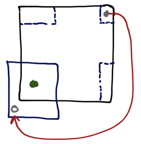
    b:(map snd (filter (\(d,_) -> d<=epsilon) dists))

The complication that arises in this code is that we want to maintain a toroidal topology for the world, so both the left and right hand sides must wrap around. Unfortunately, the KDTree as implemented assumes a flat plane that extends indefinitely in all directions. If we want to impose a toroidal topology on it, we need to do a little work. I am sure that there exist other ways to do this, but the one I quickly put together is pretty simple. The figure below should help a little in visualizing this. First, given a boid we want to query around (the green dot), we need to remap the parts of the spatial query box that fall off the world onto the other side appropriately. This allows us to capture points like the grey one that are far away in the plane sense, but nearby given the torus that we want to model. Furthermore, we need to remap the points that fall into the regions that wrap around into a coordinate system that makes sense for the boid that we are querying around. That remapping is what the red arrow corresponds to.

The code isn’t too bad to achieve this. First, we define a bounding box around the boid by defining an upper right and lower left corner. Two helpers (defined below) are used to split the bounding box horizontally, and then split the results of that vertically to yield the set of bounding boxes that we need to query. In addition to splitting the bounding boxes, we also pass around for each bounding box the adjustment that needs to be made to translate the contents of each box into the region as seen by the green boid. Once we have split the boxes and computed the offsets for each, we iterate the sequence of KDTree queries (range searches), adjust the results of each, and return the set that fall within some epsilon radius of the central boid. Note that the range search covers a rectangular region, but to maintain isotropy (direction invariance), we prune that down to a circle so that no directions are favored over others.

splitBoxHoriz :: (Vec2,Vec2,Double,Double) -> [(Vec2,Vec2,Double,Double)]
splitBoxHoriz (lo@(Vec2 lx ly), hi@(Vec2 hx hy), ax, ay) =
  if (hx-lx > w) 
  then [(Vec2 minx ly, Vec2 maxx hy, ax, ay)]
  else if (lx < minx) 
       then [(Vec2 minx ly, Vec2 hx hy, ax, ay),
             (Vec2 (maxx-(minx-lx)) ly, Vec2 maxx hy, (ax-w), ay)]
       else if (hx > maxx) 
            then [(Vec2 lx ly, Vec2 maxx hy, ax, ay),
                  (Vec2 minx ly, Vec2 (minx + (hx-maxx)) hy, ax+w, ay)]
            else [(lo,hi,ax,ay)]
  where w = maxx-minx

splitBoxVert :: (Vec2,Vec2,Double,Double) -> [(Vec2,Vec2,Double,Double)]
splitBoxVert (lo@(Vec2 lx ly), hi@(Vec2 hx hy), ax, ay) =
  if (hy-ly > h) 
  then [(Vec2 lx miny, Vec2 hx maxy, ax, ay)]
  else if (ly < miny) 
       then [(Vec2 lx miny, Vec2 hx hy, ax, ay),
             (Vec2 lx (maxy-(miny-ly)), Vec2 hx maxy, ax, ay-h)]
       else if (hy > maxy) 
            then [(Vec2 lx ly, Vec2 hx maxy, ax, ay),
                  (Vec2 lx miny, Vec2 hx (miny + (hy-maxy)), ax, ay+h)]
            else [(lo,hi,ax,ay)]
  where h = maxy-miny

That’s most of the interesting code! As mentioned above, the full program resides in github for those who wish to see further detail or try it out.

Of course, the code is only really satisfying if we can see what the output looks like. This is achieved using gloss. For example, in addition to the view above, we can observe the underlying contributors to the flocking motion, which is very useful in debugging. A video of a small number of boids running around with their epsilon regions, and alignment, cohesion, and separation vectors shown, can be seen here.

I apologize for the low quality of the video - I need to learn how to make better screen videos that don’t lose so much quality when they get uploaded to youtube (the raw files on my screen before upload look much better). A zoomed out version where the vectors are hard to resolve, but the epsilon regions are clear for a larger region with more boids can be found here.

How did this get visualized? Very simple! First, there is the code to visualize one boid.

-- some colors
boidColor       = makeColor 1.0 1.0 0.0 1.0
radiusColor     = makeColor 0.5 1.0 1.0 0.2
cohesionColor   = makeColor 1.0 0.0 0.0 1.0
separationColor = makeColor 0.0 1.0 0.0 1.0
alignmentColor  = makeColor 0.0 0.0 1.0 1.0

renderboid :: World -> Boid -> Picture
renderboid world b =
  let (Vec2 x y) = position b
      (Vec2 vx vy) = velocity b
      v = velocity b
      (Vec2 dCX dCY) = dbgC b
      (Vec2 dSX dSY) = dbgS b
      (Vec2 dAX dAY) = dbgA b
      sf = 5.0 * (scaleFactor world)
      sf' = 1.0 * (scaleFactor world)
      sf2 = sf * 10
      (xs,ys) = modelToScreen world (x,y)
      vxs = sf * (realToFrac vx) :: Float
      vys = sf * (realToFrac vy) :: Float
  in
    Pictures $ [
      Color boidColor $ 
        Translate xs ys $
        Circle 2 ,
      Color radiusColor $
        Translate xs ys $
        Circle ((realToFrac epsilon) * sf'),
      Color boidColor $          
        Line [(xs,ys), ((xs+vxs),(ys+vys))],
      Color cohesionColor $
        Line [(xs,ys), ((xs+(sf2*realToFrac dCX)),
                        (ys+(sf2*realToFrac dCY)))],
      Color alignmentColor $
        Line [(xs,ys), ((xs+(sf2*realToFrac dAX)),
                        (ys+(sf2*realToFrac dAY)))],
      Color separationColor $
        Line [(xs,ys), ((xs+(sf'*realToFrac dSX)),
                        (ys+(sf'*realToFrac dSY)))]
    ]

We see a bit of code that is used to scale vectors and positions to fit well on the screen, and then a list of visual elements that define the lines and circles along with their colors and positions. One quirk with the code is that my boid logic was based on Doubles, while Gloss uses Floats, so a necessary conversion takes place here.

Rendering the full set of boids is pretty straight forward:

renderboids :: World -> KDTreeNode Boid -> Picture
renderboids world bs = Pictures $ mapKDTree bs (renderboid world)

We also have some code that is used to map “world” coordinates to screen coordinates. This allows us to have a window that is, say, 800x800, but treat the boids as if they live in a world that spans [-4,4] in each dimension. We use a World type to pass this information around so we can do the conversion:

data World = World { width :: Double,
                     height :: Double,
                     pixWidth :: Int,
                     pixHeight :: Int } deriving Show

modelToScreen :: World -> (Double, Double) -> (Float, Float)
modelToScreen world (x,y) =
  let xscale = (fromIntegral (pixWidth world)) / (width world)
      yscale = (fromIntegral (pixHeight world)) / (height world)
  in
    (realToFrac $ x * xscale, realToFrac $ y * yscale)

scaleFactor :: World -> Float
scaleFactor world =
  let xscale = (fromIntegral (pixWidth world)) / (width world)
      yscale = (fromIntegral (pixHeight world)) / (height world)
  in
   realToFrac $ max xscale yscale

Last but not least, we have the main function that drives the whole simulation. The “simulateInWindow” function is a helper from gloss that, given window parameters, timing parameters (e.g., framerate), and a function to be called on each frame, automatically handles driving the time stepper.

main :: IO ()
main = do
  let w = World { width = (maxx-minx), height = (maxy-miny), pixWidth = 700, pixHeight = 700 }
      bs = initialize 150 10.0 0.5
      t = foldl (\t b -> kdtAddPoint t (position b) b) newKDTree bs
  simulateInWindow
    "Boids"
    (pixWidth w, pixHeight w)
    (10,10)
    (greyN 0.1)
    30 
    t
    (renderboids w)
    iterationkd

Hopefully this post is informative to people who are interested in basic algorithm visualization in Haskell, flocking algorithms, agent-based simulation, or artificial life. Please keep in mind that this is just a simple example hacked together over a weekend and tuned during the evening in my hotel room during a workshop. The code could use a significant amount of polish, but in my opinion, is at a point where people reading the post will have enough information to play with it themselves. Enjoy!