3D DLA in Haskell, Part II - Performance Tuning
About a month ago, I shared my code implementing the 3D diffusion limited aggregation algorithm. The point of that post was to show how the algorithm looked when implemented in Haskell, without any concern early on for speed. I am very interested in seeing how functional languages can be applied to computational science problems, and the DLA model seems to be an interesting example that is both short to write yet nontrivial to reason about when we work with the model in the case where we don’t restrict the random walk of the particles to a fixed grid. The use of data structures like the KDTree to perform collision detection in the absence of this fixed grid makes the code a bit more interesting to think about. Furthermore, parallelizing DLA isn’t exactly the most straightforward activity due to the changes a parallel implementation may have on the dynamics of the simulation. This talk discusses this issue a bit. I’m still going to only work with the sequential version of the algorithm for these blog posts.
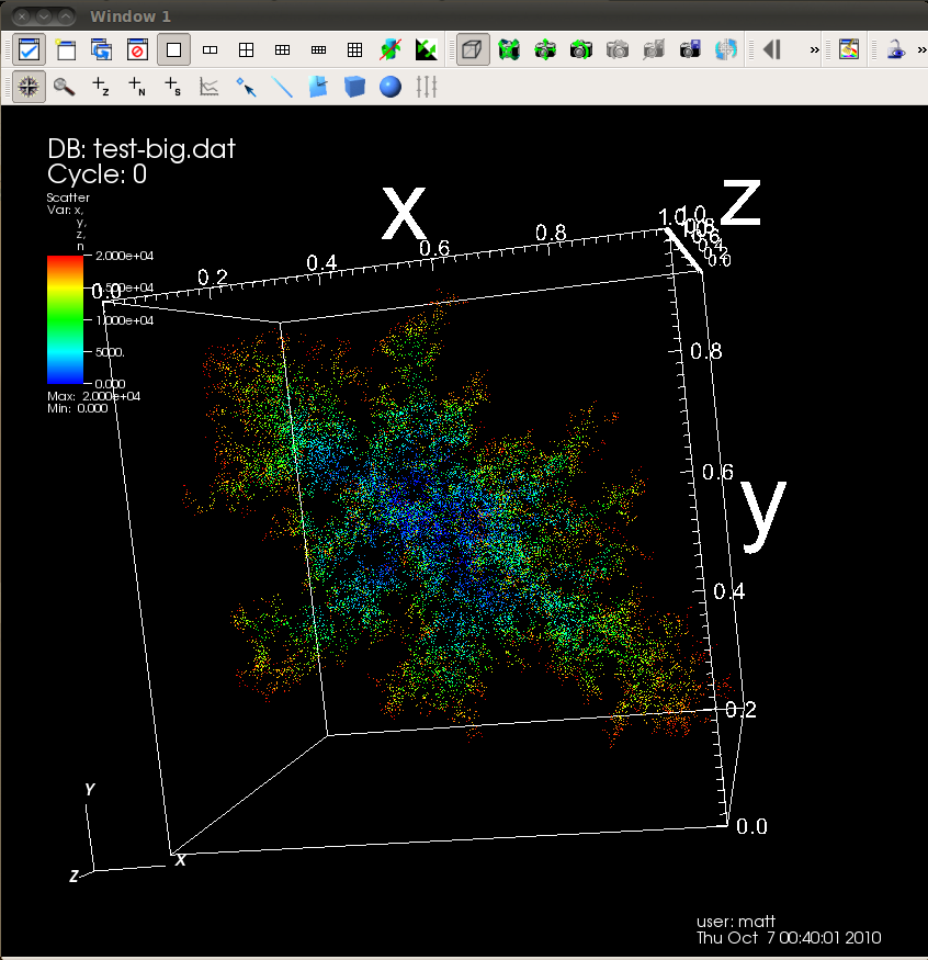
The original code ran relatively well, but compared to the C code that it was based on, it was a bit slow. I was satisfied with the readability and clarity of the code though. I promised to post a follow-up that discussed performance optimizations, and after a couple vacations and busy time at work, I’ve finally written it up. Here’s a picture of a 20,000 particle run using the optimized code. No difference is present in the output, but it took a pleasantly shorter period of time to compute!
The code was written originally with a pre-existing C code as the reference implementation. Very little deviation was made from that code, other than substituting the random number generator from the mersenne-random-pure64 package for the built in C rand() function. I was satisfied with the state of the Haskell code once it was done. It was short, easy to follow, and ran at a respectable speed. Of course, a natural thing to look at next is whether or not the Haskell code can be tuned to run a bit closer to the speed of the C code.
To do a defensible comparison, it is necessary to make the C and Haskell codes as similar as possible to start with. For example, any trick at the algorithm level that could benefit both should be applied to both. For example, I modified the original C code to call out to the same C-based code that the Mersenne-Random-Pure64 package that the Haskell code uses. Different random number generators have different performance overhead characteristics, and given that the random walk of the particles is one of the critical computations performed in the code, it only makes sense to use the same PRNG in order to eliminate any advantage or disadvantage that either side has due to that factor.
Given code that is as similar as possible to start with, we must also start with the same inputs so that both codes take similar random walks to avoid performance discrepancies due to parameter mismatches. In these experiments, we used the following parameters:
stickiness    = 1.0
death_rad     = 1.0
starting_rad  = 1.0
min_inner_rad = 1.0
inner_mult    = 2.0
outer_mult    = 1.0
curr_max_rad  = 0.0
epsilon       = 0.05
step_size     = 0.075
rng_seed      = 11
In my public github repository, there are two directories that represent the starting point for the experimentation described here. First, “unoptimized-haskell” contains the Haskell code that was described in the original post. The directory “c” contains the C code that I started from to write the unoptimized Haskell code that we began with. Seven optimizations were applied to the code incrementally so that we could see their effect on the runtime independent of each other. I did not have the patience to study their effect when applied in different orders though (that’s a few more combinations of code than I’m willing to write…).
The driver to measure the performance for all of the code versions that I wrote as I did the tuning activity was written using the Criterion package from Hackage. It’s in the repository as well, called “tester.hs”. Criterion is nice because it lets me describe the test cases that I’m interested in, and I can let it run unattended while it grinds through a number of runs in order to characterize the distribution of the runtime of each program. This post is fairly long as is, so I’ll probably post a followup about using Criterion if anyone is curious. I’d like to run a study on this code to see how the tuning relates to the different parameters, and Criterion looks like a good framework to automate the runs.
In the table below, I list the 7 different versions of the Haskell code to show the progression of performance as different optimizations are made. As we can see, most of them made an improvement (although opt3 back-pedaled a bit…). We start with a code that takes 3.93 times as long as the C code, and end up with one that takes 1.98 times as long. The last optimization, opt7, applies something to Haskell that the C code can benefit from, so the 1.68x number for comparision isn’t really fair to the C side. When the C code gets the same tweak (which we talk about later related to applying trig identities), the fastest Haskell we see takes about 2.2x the C code (called c’ in the table), and the original Haskell code takes 5.18x as much time as the final, fast C code. So, in both cases, the Haskell code that we end up with is a nice amount faster than the original.
| Version | Slowdown relative to C | Fraction of original Haskell runtime |
|---|---|---|
| Unoptimized | 3.93 | 1.0 |
| opt1 | 3.6 | 0.91 |
| opt2 | 2.79 | 0.71 |
| opt3 | 2.91 | 0.74 |
| opt4 | 2.28 | 0.57 |
| opt5 | 2.1 | 0.53 |
| opt6 | 1.98 | 0.50 |
| opt7 | 1.68 | 0.43 |
| opt7 vs c’ | 2.2 | 0.43 |
For the curious, the C code was compiled with the “-O3” optimization flags with GCC 4.4.3, and the Haskell was built using the “-O2 -fvia-C -optc-O3 -fexcess-precision” optimization flags with GHC 6.12.3. Both were run on the same 32-bit Ubuntu 10.04 machine, my Thinkpad T400. I did not spend any time tuning these flags. The C flags were just a normal one I often use, and the Haskell ones were a result of me asking someone who knows Haskell far better than me, “which flags should I use”.
opt1: Monad replacement
In this optimization, the Rmonad code was replaced with a specialized implementation of the State monad for the PureMT state only. The intent here is to give the compiler simpler code to work with in hopes that more opportunities for optimization can be found and exploited.
{-# LANGUAGE BangPatterns #-}
import System.Random.Mersenne.Pure64

data R a = R !a {-# UNPACK #-}!PureMT

newtype DLAMonad a = S { runState :: PureMT -> R a }

instance Monad DLAMonad where
    {-# INLINE return #-}
    return a = S $ \s -> R a s

    {-# INLINE (>>=) #-}
    m >>= k  = S $ \s -> case runState m s of
                                R a s' -> runState (k a) s'

    {-# INLINE (>>) #-}
    m >>  k  = S $ \s -> case runState m s of
                                R _ s' -> runState k s'

runRmonad :: DLAMonad a -> PureMT -> R a
runRmonad (S m) s = m s

nextF :: Double -> DLAMonad Double
{-# INLINE nextF #-}
nextF !up = S $ \s -> case randomDouble s of
                             (x, s') -> x `seq` R (x*up) s'
Very little should be surprising here. We have a definition of our DLAMonad that threads state of type PureMT through the code, with simple definitions of return, (>>=) and (>>). We also provide the nextF function that, given an upper bound, returns a random double that ranges from 0.0 to the bound. Each of the four functions that are used frequently are annotated with directives asking that they be inlined. Bang patters are used for the elements of the R data type in order to prevent overhead due to laziness, and the PureMT random number generator state is marked for unpacking to avoid unnecessary overhead related to its representation. This type of tuning is described in more detail here.
opt2: rem vs. mod
Examining the profile of the code at this point, we see that much of the time is being spent in the kdtRangeSearchRec function which plays a core role in collision detection.
COST CENTRE                    MODULE               %time %alloc

kdtRangeSearchRec              DLA.KDTree            18.9   27.2
vecDimSelect                   DLA.Vec3              18.2    8.1
nextF                          DLA.Rmonad            12.5   17.6
>>=_a2tt                       DLA.Rmonad            10.3    7.2
randVec                        DLA.Vec3               9.3    9.6
kdtCollisionDetect             DLA.KDTree             8.4   10.6
vecLessThan                    DLA.Vec3               5.0    4.4
walk_particle                  Main                   4.8    3.7
runState                       DLA.Rmonad             2.4    0.0
sticks                         Main                   2.3    1.1
vecAdd                         DLA.Vec3               1.8    1.9
return_a2tQ                    DLA.Rmonad             1.8    2.8
vecDot                         DLA.Vec3               1.5    2.6
kdtInBounds                    DLA.KDTree             0.8    1.7
This is because each step the particle takes, two things happen – we sample the random number source, and then have to check the KDTree to see if the particle will collide with any others that have already joined in the aggregate. In a KDTree, this is accomplished by drilling down into the tree to see if any particles are in it already that are within some sphere of a given radius. Therefore we heavily use the kdtRangeSearchRec function for searching for particles within a given cube (from which we will look at the sphere embedded in the cube to make sure we didn’t only see points in the corners of the cube that are slightly out of reach). Each call to kdtRangeSearchRec calls vecDimSelect multiple times to look at the appropriate element of the vectors representing the position and the bounding box of the cube.
I am originally a programmer from the C world, and when I see code that reads “x % 42”, I read this as “X mod forty-two”. It shouldn’t be a surprise that when translating the vecDimSelect code to Haskell, when I said that in my mind as I read the C code I translated it to what I thought was the equivalent function in Haskell called “mod”. That turns out to not be correct. Consider the following:
Which of these matches the behavior of % in C? ‘rem’ does. It turns out that mod is slower due to a sign check that rem doesn’t perform. For positive numbers the two are the same. In our case, the KDTree functions that need to compute which dimension they are working with based on a positive depth counter can get away with both — so why not use the faster one? The change to vecDimSelect is simple, and results in a slight speedup.
opt3: vecDimSelect
Upon closer examination to vecDimSelect, we would actually like to try to avoid doing the rem at all and just return the element of the vector that we need without any computation. If we know the dimension of the vectors that we are working with, we can change the recursive tree traversal to not pass the increasing depth forward with each call, but instead check to see if the depth is within the range we want for the vector dimension, and manually flip it over to 0 to start over when it exceeds the acceptable range. In our 3D case, this means flipping it over when we’re about to increment it to 3. Consider the code for adding a particle after we’ve applied this:
kdtAddWithDepth (Node left npos ndata right) pos dat d =
  if (vecDimSelect pos d) < (vecDimSelect npos d) then
    Node (kdtAddWithDepth left pos dat d') npos ndata right
  else
    Node left npos ndata (kdtAddWithDepth right pos dat d')
  where d' = if (d == 2) then 0 else d+1
Instead of calling the function recursively with a depth d+1, we compute d’ in the where clause not using rem or mod or any numerical function, but a simple conditional. This same trick can be applied to kdtRangeSearchRec. This then allows us to rewrite the vecDimSelect function to no longer use the rem unless a value greater than 2 is passed in.
vecDimSelect :: Vec3 -> Int -> Double
{-# INLINE vecDimSelect #-}
vecDimSelect (Vec3 a b c) n =
  case n of
    0 -> a
    1 -> b
    2 -> c
    _ -> case (rem n 3) of
           0 -> a
           1 -> b
           2 -> c
This simple change had a negligible impact on performance though.
opt4: eliminate vecdimselect
Examining the profile, we still see that vecDimSelect is a bit of an annoyance and consumes noticable time. At this point of the tuning process, I realized that it was time to see if vecDimSelect could be ejected entirely from the logic for the range search code. The change I perform to do this is one in which I give up conciseness in the code in exchange for speed. To make the vecDimSelect call go away, I manually unroll the recursive function to create three functions specialized to each of the three dimensions of the vectors. These then mutually call each other in a cycle, avoiding the need to pass depths around entirely. During this process, I also realized that the Leaf was redundant in the KDTree data structure (somehow that slipped by me), and I replaced it with the more concise structure that contains simply Nodes and Empties. That change had no effect on the performance that I could notice, but did simplify the code.
The range search code changes from:
kdtRangeSearchRec (Node left npos ndata right) bMin bMax d =
  if (vecDimSelect npos d) < (vecDimSelect bMin d) then
    kdtRangeSearchRec right bMin bMax d'
  else
    if (vecDimSelect npos d) > (vecDimSelect bMax d) then
      kdtRangeSearchRec left bMin bMax d'
    else
      if (kdtInBounds npos bMin bMax) then
        (npos,ndata) : ((kdtRangeSearchRec right bMin bMax d')++
                        (kdtRangeSearchRec left bMin bMax d'))
      else
        (kdtRangeSearchRec right bMin bMax d')++
        (kdtRangeSearchRec left bMin bMax d')
  where d' = if (d == 2) then 0 else d+1

kdtRangeSearch :: (KDTreeNode a) -> Vec3 -> Vec3 -> [(Vec3,a)]
kdtRangeSearch t bMin bMax =
  kdtRangeSearchRec t bMin bMax 0
To:
-- X dimension
kdtRangeSearchRecX :: (KDTreeNode a) -> Vec3 -> Vec3 -> [(Vec3,a)]
kdtRangeSearchRecX Empty _ _ = []
kdtRangeSearchRecX (Node left npos ndata right) bMin bMax =
  if nc < mnc then
    nextfun right bMin bMax
  else
    if nc > mxc then
      nextfun left bMin bMax
    else
      if (kdtInBounds npos bMin bMax) then
        (npos,ndata) : ((nextfun right bMin bMax)++
                        (nextfun left bMin bMax))
      else
        (nextfun right bMin bMax)++
        (nextfun left bMin bMax)
  where Vec3 nc _ _  = npos
        Vec3 mnc _ _ = bMin
        Vec3 mxc _ _ = bMax
        nextfun = kdtRangeSearchRecY

-- Y dimension
kdtRangeSearchRecY :: (KDTreeNode a) -> Vec3 -> Vec3 -> [(Vec3,a)]
kdtRangeSearchRecY Empty _ _ = []
kdtRangeSearchRecY (Node left npos ndata right) bMin bMax =
  if nc < mnc then
    nextfun right bMin bMax
  else
    if nc > mxc then
      nextfun left bMin bMax
    else
      if (kdtInBounds npos bMin bMax) then
        (npos,ndata) : ((nextfun right bMin bMax)++
                        (nextfun left bMin bMax))
      else
        (nextfun right bMin bMax)++
        (nextfun left bMin bMax)
  where Vec3 _ nc _  = npos
        Vec3 _ mnc _ = bMin
        Vec3 _ mxc _ = bMax
        nextfun = kdtRangeSearchRecZ

-- Z dimension
kdtRangeSearchRecZ :: (KDTreeNode a) -> Vec3 -> Vec3 -> [(Vec3,a)]
kdtRangeSearchRecZ Empty _ _ = []
kdtRangeSearchRecZ (Node left npos ndata right) bMin bMax =
  if nc < mnc then
    nextfun right bMin bMax
  else
    if nc > mxc then
      nextfun left bMin bMax
    else
      if (kdtInBounds npos bMin bMax) then
        (npos,ndata) : ((nextfun right bMin bMax)++
                        (nextfun left bMin bMax))
      else
        (nextfun right bMin bMax)++
        (nextfun left bMin bMax)
  where Vec3 _ _ nc  = npos
        Vec3 _ _ mnc = bMin
        Vec3 _ _ mxc = bMax
        nextfun = kdtRangeSearchRecX

kdtRangeSearch :: (KDTreeNode a) -> Vec3 -> Vec3 -> [(Vec3,a)]
kdtRangeSearch t bMin bMax =
  kdtRangeSearchRecX t bMin bMax
This code is a bit longer, but the result on performance is quite nice. It should be noted that as a result of this change, we are also performing common subexpression elimination by hand. In the original code, we made two calls to vecDimSelect to select the same component of the node position. It turns out that my replication of code with an assumption that the compiler would perform common subexpression elimination was another legacy of the programming habits I picked up as a C programmer. As you can see on this page, GHC does not perform as much CSE as one might expect coming from other languages due to the potential for space leaks that CSE can introduce. This was an interesting thing to learn that I hadn’t encountered previously (if it was in some of the books I read when learning Haskell, I missed it.)
opt5: more cse, more bang patterns
At this point I realized that some of the optimizations applied to the KDTree and Rmonad could be applied elsewhere. I did a quick scan over the code to make sure I hadn’t made any other assumptions about the compiler doing CSE for me, and looked carefully at the Vec3 code to see if bang patterns could be applied to speed up those functions. The modified Vec3 was pretty simple. The changes are shown below:
import DLA.Rmonad

data Vec3 = Vec3 !Double !Double !Double

randVec :: Double -> DLAMonad Vec3
randVec r = do
  phi <- nextF (2.0 * pi)  -- phi ranges from 0.0 to 2.0*pi
  z <- nextF (2.0 * r)
  let z' = z - r    -- z ranges from -r to r
  let rct = r * cos ( asin (z' / r) )
  return $ Vec3 (rct*(cos phi)) (rct*(sin phi)) z'

vecScale :: Vec3 -> Double -> Vec3
vecScale (Vec3 a b c) !s = Vec3 (a*s) (b*s) (c*s)
The rest of the functions remained untouched. The contents of the Vector data type are made strict, as is the Double parameter to vecScale. Common subexpression elimination is applied to randVec to roll what used to be the computation of
\[\theta=\arcsin(z/r)\]
and
\[ r*\cos(\theta)\]
into a single computation which is reused twice when forming the vector to return.
opt6: more bang patterns
The next optimization I tried was to see if this same gain could be seen within the KDTree. So far, optimizations to the KDTree code focused on high level function structure and algorithms, and less on things like lazy versus strict evaluation. It turns out that, while these do contribute some to the overall optimization improvement, the contribution is tiny. Applying bang patterns and making the KDTree data type have strict contents didn’t do much.
Thinking this through though, it makes sense. For example, if we run a simulation with 2000 particles, we expect that the KDTree will have at most 2000 nodes. This is only 2000 objects of type KDTNode. On the other hand, vectors are created and destroyed many more times. Looking at the profile for a 2000 particle simulation, we see 1122563 random vectors generated. Therefore if we were to suffer some overhead due to laziness for each object that is created, there would be a much higher contribution of overhead from the far higher number of vector objects that come and go.
opt7: Reducing floating point operations
One blog commenter pointed out an identity that had been long purged from my brain (likely in one of my moments in high school when calculus was a source of much unpleasantness – I didn’t learn to like Math until I hit abstract algebra in college). This identity is:
\[ \cos(\arcsin(z)) = \sqrt{1-z^2}\]
This is appealing because it reduces the floating point overhead for the random vector generation code a great deal. Given that randVec is called quite a bit, this is a large amount of potential savings. This was an optimization that required more thought though than the others because, not only did it require testing to see how it sped up the code, it required more testing to make sure it didn’t damage the code.
The reason for this is that for the other versions, “diff” was sufficient to verify that the changes weren’t breaking the code. They were producing EXACTLY the same output. With this new change though, diff failed. It turns out, there are subtle differences due to differences in the floating point operations performed, but the errors introduced are down in the 10^-16 scale. This was worrying though - small errors can accumulate and be quite disruptive. I tried to see if this change was harmless (which it appears to be) by two tests - one qualitative, one quantitative.
The qualitative test was easy - run the code from before and after the change for a substantial number of particles, and see if the accumulated error causes the structure to change as it grows. No noticeable difference in the plots as visualized. Of course, the “by eye” test is dangerous, so I wrote a simple test program that was intended to show errors blowing up if they were in fact accumulating. I just wrote a program that takes a random walk for a number of steps, where small perturbations at each step should get amplified as the walk goes on.
import Vec3
import Rmonad
import System.Random.Mersenne.Pure64

vecZero :: Vec3
vecZero = Vec3 0.0 0.0 0.0

stepsize :: Double
stepsize = 1.0

walker :: Vec3 -> Int -> (Double -> DLAMonad Vec3) -> DLAMonad [Vec3]
walker v 0 rv = return [v]
walker v n rv = do
  s <- rv stepsize
  slist <- (walker s (n-1) rv)
  return (v:slist)

walk :: Int -> (Double -> DLAMonad Vec3) -> DLAMonad [Vec3]
walk n rv = walker vecZero n rv

main :: IO ()
main = do
  let R s _ = runRmonad (walk 100000 randVec) (pureMT 10)
  let R s' _ = runRmonad (walk 100000 randVecNew) (pureMT 10)

  junk <- mapM (\(v1,v2) -> putStrLn $ show $ vecNorm $ vecSub v1 v2) (zip s s')
  return ()
The output of this program is a series of numbers representing the difference in position of the walk at each point. Looking at the data in Octave, I don’t see any growth - the mean stays around 10^-17, and rarely is above 10^-16. This looks like floating point noise to me with numbers down in the “essentially zero” range.
This was the last change I made, and made it to the C code as well. The final time taken by the optimized Haskell code (opt7) was 2.2x the C code with this applied, and 1.68x the C code without it. This is a nice improvement over the original Haskell code which took 5.18x and 3.93x as long as the C codes.
Hopefully this was somewhat informative. I’ll probably follow up with some more experiments with this code and some info on how I used Criterion to do some performance studies.
10/10/10 Edits: based on comments, I’ve updated the code above from the original post to use proper let notation in the randVec code. I also reduced the number of samples in the quick test code I wrote to probe the potential error accumulation between the two randVec implementations. A larger number will require you to increase the stack size or use the code from the commenter who pointed out the issue.